A demo of K-Means clustering on the handwritten digits data

In this example we compare the various initialization strategies for K-means in terms of runtime and quality of the results.

As the ground truth is known here, we also apply different cluster quality metrics to judge the goodness of fit of the cluster labels to the ground truth.

Cluster quality metrics evaluated (see Clustering performance evaluation for definitions and discussions of the metrics):

Shorthand	full name
homo	homogeneity score
compl	completeness score
v-meas	V measure
ARI	adjusted Rand index
AMI	adjusted mutual information
silhouette	silhouette coefficient

Script output:

n_digits: 10,    n_samples 1797,         n_features 64
_______________________________________________________________________________
init    time  inertia    homo   compl  v-meas     ARI AMI  silhouette
k-means++   0.64s    69432   0.602   0.650   0.625   0.465   0.598    0.146
   random   0.65s    69694   0.669   0.710   0.689   0.553   0.666    0.147
PCA-based   0.05s    71820   0.673   0.715   0.693   0.567   0.670    0.150
_______________________________________________________________________________

Python source code: plot_kmeans_digits.py

print(__doc__)

from time import time
import numpy as np
import matplotlib.pyplot as plt

from sklearn import metrics
from sklearn.cluster import KMeans
from sklearn.datasets import load_digits
from sklearn.decomposition import PCA
from sklearn.preprocessing import scale

np.random.seed(42)

digits = load_digits()
data = scale(digits.data)

n_samples, n_features = data.shape
n_digits = len(np.unique(digits.target))
labels = digits.target

sample_size = 300

print("n_digits: %d, \t n_samples %d, \t n_features %d"
      % (n_digits, n_samples, n_features))


print(79 * '_')
print('% 9s' % 'init'
      '    time  inertia    homo   compl  v-meas     ARI AMI  silhouette')


def bench_k_means(estimator, name, data):
    t0 = time()
    estimator.fit(data)
    print('% 9s   %.2fs    %i   %.3f   %.3f   %.3f   %.3f   %.3f    %.3f'
          % (name, (time() - t0), estimator.inertia_,
             metrics.homogeneity_score(labels, estimator.labels_),
             metrics.completeness_score(labels, estimator.labels_),
             metrics.v_measure_score(labels, estimator.labels_),
             metrics.adjusted_rand_score(labels, estimator.labels_),
             metrics.adjusted_mutual_info_score(labels,  estimator.labels_),
             metrics.silhouette_score(data, estimator.labels_,
                                      metric='euclidean',
                                      sample_size=sample_size)))

bench_k_means(KMeans(init='k-means++', n_clusters=n_digits, n_init=10),
              name="k-means++", data=data)

bench_k_means(KMeans(init='random', n_clusters=n_digits, n_init=10),
              name="random", data=data)

# in this case the seeding of the centers is deterministic, hence we run the
# kmeans algorithm only once with n_init=1
pca = PCA(n_components=n_digits).fit(data)
bench_k_means(KMeans(init=pca.components_, n_clusters=n_digits, n_init=1),
              name="PCA-based",
              data=data)
print(79 * '_')

###############################################################################
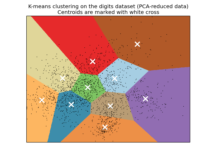
# Visualize the results on PCA-reduced data

reduced_data = PCA(n_components=2).fit_transform(data)
kmeans = KMeans(init='k-means++', n_clusters=n_digits, n_init=10)
kmeans.fit(reduced_data)

# Step size of the mesh. Decrease to increase the quality of the VQ.
h = .02     # point in the mesh [x_min, m_max]x[y_min, y_max].

# Plot the decision boundary. For that, we will assign a color to each
x_min, x_max = reduced_data[:, 0].min() + 1, reduced_data[:, 0].max() - 1
y_min, y_max = reduced_data[:, 1].min() + 1, reduced_data[:, 1].max() - 1
xx, yy = np.meshgrid(np.arange(x_min, x_max, h), np.arange(y_min, y_max, h))

# Obtain labels for each point in mesh. Use last trained model.
Z = kmeans.predict(np.c_[xx.ravel(), yy.ravel()])

# Put the result into a color plot
Z = Z.reshape(xx.shape)
plt.figure(1)
plt.clf()
plt.imshow(Z, interpolation='nearest',
           extent=(xx.min(), xx.max(), yy.min(), yy.max()),
           cmap=plt.cm.Paired,
           aspect='auto', origin='lower')

plt.plot(reduced_data[:, 0], reduced_data[:, 1], 'k.', markersize=2)
# Plot the centroids as a white X
centroids = kmeans.cluster_centers_
plt.scatter(centroids[:, 0], centroids[:, 1],
            marker='x', s=169, linewidths=3,
            color='w', zorder=10)
plt.title('K-means clustering on the digits dataset (PCA-reduced data)\n'
          'Centroids are marked with white cross')
plt.xlim(x_min, x_max)
plt.ylim(y_min, y_max)
plt.xticks(())
plt.yticks(())
plt.show()

Total running time of the example: 2.19 seconds ( 0 minutes 2.19 seconds)