sklearn.linear_model.lasso_path
- sklearn.linear_model.lasso_path(X, y, eps=0.001, n_alphas=100, alphas=None, precompute='auto', Xy=None, fit_intercept=None, normalize=None, copy_X=True, coef_init=None, verbose=False, return_models=False, **params)
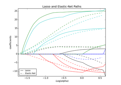
Compute Lasso path with coordinate descent
The Lasso optimization function varies for mono and multi-outputs.
For mono-output tasks it is:
(1 / (2 * n_samples)) * ||y - Xw||^2_2 + alpha * ||w||_1
For multi-output tasks it is:
(1 / (2 * n_samples)) * ||Y - XW||^2_Fro + alpha * ||W||_21
Where:
||W||_21 = \sum_i \sqrt{\sum_j w_{ij}^2}i.e. the sum of norm of each row.
Parameters: X : {array-like, sparse matrix}, shape (n_samples, n_features)
Training data. Pass directly as Fortran-contiguous data to avoid unnecessary memory duplication. If y is mono-output then X can be sparse.
y : ndarray, shape = (n_samples,), or (n_samples, n_outputs)
Target values
eps : float, optional
Length of the path. eps=1e-3 means that alpha_min / alpha_max = 1e-3
n_alphas : int, optional
Number of alphas along the regularization path
alphas : ndarray, optional
List of alphas where to compute the models. If None alphas are set automatically
precompute : True | False | ‘auto’ | array-like
Whether to use a precomputed Gram matrix to speed up calculations. If set to 'auto' let us decide. The Gram matrix can also be passed as argument.
Xy : array-like, optional
Xy = np.dot(X.T, y) that can be precomputed. It is useful only when the Gram matrix is precomputed.
fit_intercept : bool
Fit or not an intercept. WARNING : deprecated, will be removed in 0.16.
normalize : boolean, optional, default False
If True, the regressors X will be normalized before regression. WARNING : deprecated, will be removed in 0.16.
copy_X : boolean, optional, default True
If True, X will be copied; else, it may be overwritten.
coef_init : array, shape (n_features, ) | None
The initial values of the coefficients.
verbose : bool or integer
Amount of verbosity.
return_models : boolean, optional, default True
If True, the function will return list of models. Setting it to False will change the function output returning the values of the alphas and the coefficients along the path. Returning the model list will be removed in version 0.16.
params : kwargs
keyword arguments passed to the coordinate descent solver.
Returns: models : a list of models along the regularization path
(Is returned if return_models is set True (default).
alphas : array, shape (n_alphas,)
The alphas along the path where models are computed. (Is returned, along with coefs, when return_models is set to False)
coefs : array, shape (n_features, n_alphas) or
(n_outputs, n_features, n_alphas)
Coefficients along the path. (Is returned, along with alphas, when return_models is set to False).
dual_gaps : array, shape (n_alphas,)
The dual gaps at the end of the optimization for each alpha. (Is returned, along with alphas, when return_models is set to False).
See also
lars_path, Lasso, LassoLars, LassoCV, LassoLarsCV, sklearn.decomposition.sparse_encode
Notes
See examples/linear_model/plot_lasso_coordinate_descent_path.py for an example.
To avoid unnecessary memory duplication the X argument of the fit method should be directly passed as a Fortran-contiguous numpy array.
Note that in certain cases, the Lars solver may be significantly faster to implement this functionality. In particular, linear interpolation can be used to retrieve model coefficients between the values output by lars_path
Deprecation Notice: Setting return_models to False will make the Lasso Path return an output in the style used by lars_path. This will be become the norm as of version 0.16. Leaving return_models set to True will let the function return a list of models as before.
Examples
Comparing lasso_path and lars_path with interpolation:
>>> X = np.array([[1, 2, 3.1], [2.3, 5.4, 4.3]]).T
>>> y = np.array([1, 2, 3.1])
>>> # Use lasso_path to compute a coefficient path
>>> _, coef_path, _ = lasso_path(X, y, alphas=[5., 1., .5],
...                              fit_intercept=False)
>>> print(coef_path)
[[ 0.          0.          0.46874778]
 [ 0.2159048   0.4425765   0.23689075]]
>>> # Now use lars_path and 1D linear interpolation to compute the
>>> # same path
>>> from sklearn.linear_model import lars_path
>>> alphas, active, coef_path_lars = lars_path(X, y, method='lasso')
>>> from scipy import interpolate
>>> coef_path_continuous = interpolate.interp1d(alphas[::-1],
...                                             coef_path_lars[:, ::-1])
>>> print(coef_path_continuous([5., 1., .5]))
[[ 0.          0.          0.46915237]
 [ 0.2159048   0.4425765   0.23668876]]