RBF SVM parameters

This example illustrates the effect of the parameters gamma and C of the rbf kernel SVM.

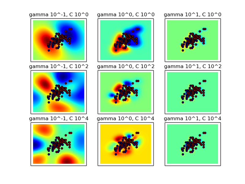
Intuitively, the gamma parameter defines how far the influence of a single training example reaches, with low values meaning ‘far’ and high values meaning ‘close’. The C parameter trades off misclassification of training examples against simplicity of the decision surface. A low C makes the decision surface smooth, while a high C aims at classifying all training examples correctly.

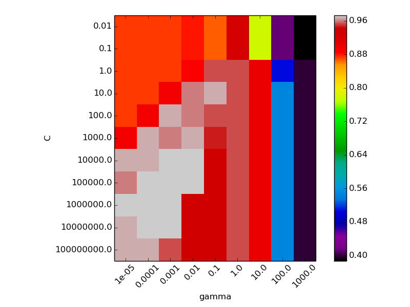
Two plots are generated. The first is a visualization of the decision function for a variety of parameter values, and the second is a heatmap of the classifier’s cross-validation accuracy as a function of C and gamma. For this example we explore a relatively large grid for illustration purposes. In practice, a logarithmic grid from 10**-3 to 10**3 is usually sufficient.

• 
• 

Script output:

The best classifier is:  SVC(C=10000.0, cache_size=200, class_weight=None, coef0=0.0, degree=3,
  gamma=0.001, kernel='rbf', max_iter=-1, probability=False,
  random_state=None, shrinking=True, tol=0.001, verbose=False)

Python source code: plot_rbf_parameters.py

print(__doc__)

import numpy as np
import matplotlib.pyplot as plt

from sklearn.svm import SVC
from sklearn.preprocessing import StandardScaler
from sklearn.datasets import load_iris
from sklearn.cross_validation import StratifiedKFold
from sklearn.grid_search import GridSearchCV

##############################################################################
# Load and prepare data set
#
# dataset for grid search
iris = load_iris()
X = iris.data
Y = iris.target

# dataset for decision function visualization
X_2d = X[:, :2]
X_2d = X_2d[Y > 0]
Y_2d = Y[Y > 0]
Y_2d -= 1

# It is usually a good idea to scale the data for SVM training.
# We are cheating a bit in this example in scaling all of the data,
# instead of fitting the transformation on the training set and
# just applying it on the test set.

scaler = StandardScaler()

X = scaler.fit_transform(X)
X_2d = scaler.fit_transform(X_2d)

##############################################################################
# Train classifier
#
# For an initial search, a logarithmic grid with basis
# 10 is often helpful. Using a basis of 2, a finer
# tuning can be achieved but at a much higher cost.

C_range = 10.0 ** np.arange(-2, 9)
gamma_range = 10.0 ** np.arange(-5, 4)
param_grid = dict(gamma=gamma_range, C=C_range)
cv = StratifiedKFold(y=Y, n_folds=3)
grid = GridSearchCV(SVC(), param_grid=param_grid, cv=cv)
grid.fit(X, Y)

print("The best classifier is: ", grid.best_estimator_)

# Now we need to fit a classifier for all parameters in the 2d version
# (we use a smaller set of parameters here because it takes a while to train)
C_2d_range = [1, 1e2, 1e4]
gamma_2d_range = [1e-1, 1, 1e1]
classifiers = []
for C in C_2d_range:
    for gamma in gamma_2d_range:
        clf = SVC(C=C, gamma=gamma)
        clf.fit(X_2d, Y_2d)
        classifiers.append((C, gamma, clf))

##############################################################################
# visualization
#
# draw visualization of parameter effects
plt.figure(figsize=(8, 6))
xx, yy = np.meshgrid(np.linspace(-5, 5, 200), np.linspace(-5, 5, 200))
for (k, (C, gamma, clf)) in enumerate(classifiers):
    # evaluate decision function in a grid
    Z = clf.decision_function(np.c_[xx.ravel(), yy.ravel()])
    Z = Z.reshape(xx.shape)

    # visualize decision function for these parameters
    plt.subplot(len(C_2d_range), len(gamma_2d_range), k + 1)
    plt.title("gamma 10^%d, C 10^%d" % (np.log10(gamma), np.log10(C)),
              size='medium')

    # visualize parameter's effect on decision function
    plt.pcolormesh(xx, yy, -Z, cmap=plt.cm.jet)
    plt.scatter(X_2d[:, 0], X_2d[:, 1], c=Y_2d, cmap=plt.cm.jet)
    plt.xticks(())
    plt.yticks(())
    plt.axis('tight')

# plot the scores of the grid
# grid_scores_ contains parameter settings and scores
score_dict = grid.grid_scores_

# We extract just the scores
scores = [x[1] for x in score_dict]
scores = np.array(scores).reshape(len(C_range), len(gamma_range))

# draw heatmap of accuracy as a function of gamma and C
plt.figure(figsize=(8, 6))
plt.subplots_adjust(left=0.05, right=0.95, bottom=0.15, top=0.95)
plt.imshow(scores, interpolation='nearest', cmap=plt.cm.spectral)
plt.xlabel('gamma')
plt.ylabel('C')
plt.colorbar()
plt.xticks(np.arange(len(gamma_range)), gamma_range, rotation=45)
plt.yticks(np.arange(len(C_range)), C_range)

plt.show()

Total running time of the example: 2.37 seconds ( 0 minutes 2.37 seconds)