Note

Go to the end to download the full example code or to run this example in your browser via JupyterLite or Binder

Single estimator versus bagging: bias-variance decomposition¶

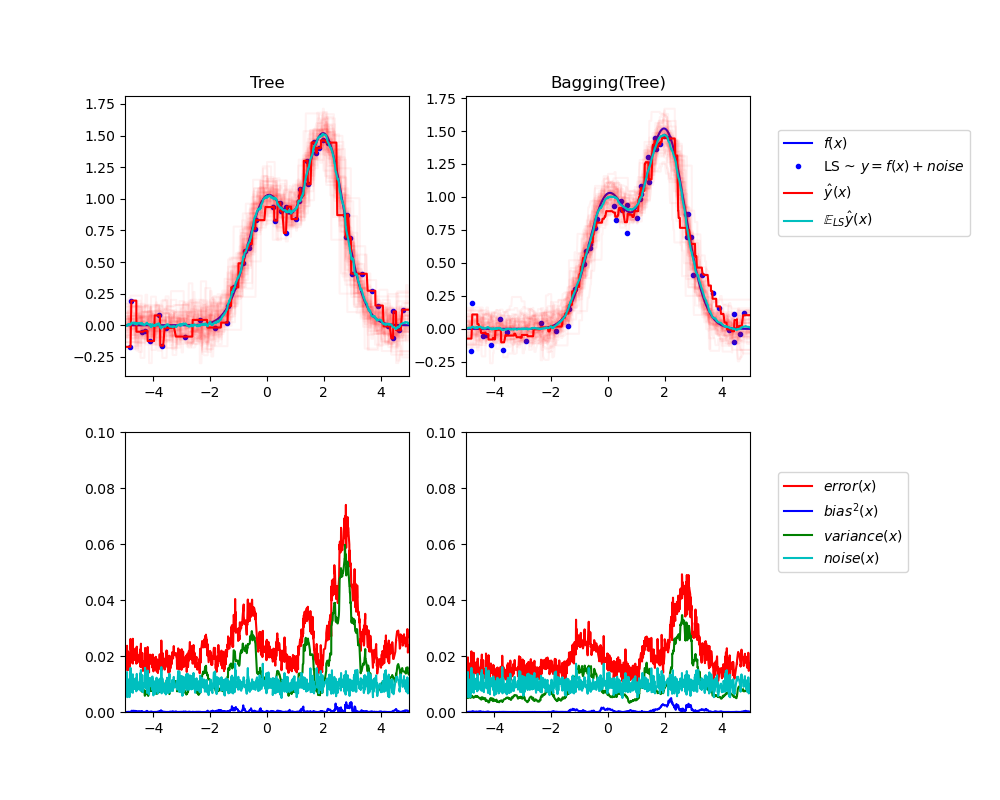
This example illustrates and compares the bias-variance decomposition of the expected mean squared error of a single estimator against a bagging ensemble.

In regression, the expected mean squared error of an estimator can be decomposed in terms of bias, variance and noise. On average over datasets of the regression problem, the bias term measures the average amount by which the predictions of the estimator differ from the predictions of the best possible estimator for the problem (i.e., the Bayes model). The variance term measures the variability of the predictions of the estimator when fit over different random instances of the same problem. Each problem instance is noted “LS”, for “Learning Sample”, in the following. Finally, the noise measures the irreducible part of the error which is due the variability in the data.

The upper left figure illustrates the predictions (in dark red) of a single decision tree trained over a random dataset LS (the blue dots) of a toy 1d regression problem. It also illustrates the predictions (in light red) of other single decision trees trained over other (and different) randomly drawn instances LS of the problem. Intuitively, the variance term here corresponds to the width of the beam of predictions (in light red) of the individual estimators. The larger the variance, the more sensitive are the predictions for x to small changes in the training set. The bias term corresponds to the difference between the average prediction of the estimator (in cyan) and the best possible model (in dark blue). On this problem, we can thus observe that the bias is quite low (both the cyan and the blue curves are close to each other) while the variance is large (the red beam is rather wide).

The lower left figure plots the pointwise decomposition of the expected mean squared error of a single decision tree. It confirms that the bias term (in blue) is low while the variance is large (in green). It also illustrates the noise part of the error which, as expected, appears to be constant and around 0.01.

The right figures correspond to the same plots but using instead a bagging ensemble of decision trees. In both figures, we can observe that the bias term is larger than in the previous case. In the upper right figure, the difference between the average prediction (in cyan) and the best possible model is larger (e.g., notice the offset around x=2). In the lower right figure, the bias curve is also slightly higher than in the lower left figure. In terms of variance however, the beam of predictions is narrower, which suggests that the variance is lower. Indeed, as the lower right figure confirms, the variance term (in green) is lower than for single decision trees. Overall, the bias- variance decomposition is therefore no longer the same. The tradeoff is better for bagging: averaging several decision trees fit on bootstrap copies of the dataset slightly increases the bias term but allows for a larger reduction of the variance, which results in a lower overall mean squared error (compare the red curves int the lower figures). The script output also confirms this intuition. The total error of the bagging ensemble is lower than the total error of a single decision tree, and this difference indeed mainly stems from a reduced variance.

For further details on bias-variance decomposition, see section 7.3 of [1].

References¶

Tree: 0.0255 (error) = 0.0003 (bias^2)  + 0.0152 (var) + 0.0098 (noise)
Bagging(Tree): 0.0196 (error) = 0.0004 (bias^2)  + 0.0092 (var) + 0.0098 (noise)

# Author: Gilles Louppe <g.louppe@gmail.com>
# License: BSD 3 clause

import matplotlib.pyplot as plt
import numpy as np

from sklearn.ensemble import BaggingRegressor
from sklearn.tree import DecisionTreeRegressor

# Settings
n_repeat = 50  # Number of iterations for computing expectations
n_train = 50  # Size of the training set
n_test = 1000  # Size of the test set
noise = 0.1  # Standard deviation of the noise
np.random.seed(0)

# Change this for exploring the bias-variance decomposition of other
# estimators. This should work well for estimators with high variance (e.g.,
# decision trees or KNN), but poorly for estimators with low variance (e.g.,
# linear models).
estimators = [
    ("Tree", DecisionTreeRegressor()),
    ("Bagging(Tree)", BaggingRegressor(DecisionTreeRegressor())),
]

n_estimators = len(estimators)


# Generate data
def f(x):
    x = x.ravel()

    return np.exp(-(x**2)) + 1.5 * np.exp(-((x - 2) ** 2))


def generate(n_samples, noise, n_repeat=1):
    X = np.random.rand(n_samples) * 10 - 5
    X = np.sort(X)

    if n_repeat == 1:
        y = f(X) + np.random.normal(0.0, noise, n_samples)
    else:
        y = np.zeros((n_samples, n_repeat))

        for i in range(n_repeat):
            y[:, i] = f(X) + np.random.normal(0.0, noise, n_samples)

    X = X.reshape((n_samples, 1))

    return X, y


X_train = []
y_train = []

for i in range(n_repeat):
    X, y = generate(n_samples=n_train, noise=noise)
    X_train.append(X)
    y_train.append(y)

X_test, y_test = generate(n_samples=n_test, noise=noise, n_repeat=n_repeat)

plt.figure(figsize=(10, 8))

# Loop over estimators to compare
for n, (name, estimator) in enumerate(estimators):
    # Compute predictions
    y_predict = np.zeros((n_test, n_repeat))

    for i in range(n_repeat):
        estimator.fit(X_train[i], y_train[i])
        y_predict[:, i] = estimator.predict(X_test)

    # Bias^2 + Variance + Noise decomposition of the mean squared error
    y_error = np.zeros(n_test)

    for i in range(n_repeat):
        for j in range(n_repeat):
            y_error += (y_test[:, j] - y_predict[:, i]) ** 2

    y_error /= n_repeat * n_repeat

    y_noise = np.var(y_test, axis=1)
    y_bias = (f(X_test) - np.mean(y_predict, axis=1)) ** 2
    y_var = np.var(y_predict, axis=1)

    print(
        "{0}: {1:.4f} (error) = {2:.4f} (bias^2) "
        " + {3:.4f} (var) + {4:.4f} (noise)".format(
            name, np.mean(y_error), np.mean(y_bias), np.mean(y_var), np.mean(y_noise)
        )
    )

    # Plot figures
    plt.subplot(2, n_estimators, n + 1)
    plt.plot(X_test, f(X_test), "b", label="$f(x)$")
    plt.plot(X_train[0], y_train[0], ".b", label="LS ~ $y = f(x)+noise$")

    for i in range(n_repeat):
        if i == 0:
            plt.plot(X_test, y_predict[:, i], "r", label=r"$\^y(x)$")
        else:
            plt.plot(X_test, y_predict[:, i], "r", alpha=0.05)

    plt.plot(X_test, np.mean(y_predict, axis=1), "c", label=r"$\mathbb{E}_{LS} \^y(x)$")

    plt.xlim([-5, 5])
    plt.title(name)

    if n == n_estimators - 1:
        plt.legend(loc=(1.1, 0.5))

    plt.subplot(2, n_estimators, n_estimators + n + 1)
    plt.plot(X_test, y_error, "r", label="$error(x)$")
    plt.plot(X_test, y_bias, "b", label="$bias^2(x)$"),
    plt.plot(X_test, y_var, "g", label="$variance(x)$"),
    plt.plot(X_test, y_noise, "c", label="$noise(x)$")

    plt.xlim([-5, 5])
    plt.ylim([0, 0.1])

    if n == n_estimators - 1:
        plt.legend(loc=(1.1, 0.5))

plt.subplots_adjust(right=0.75)
plt.show()