Label Propagation digits: Demonstrating performance

This example demonstrates the power of semisupervised learning by training a Label Spreading model to classify handwritten digits with sets of very few labels.

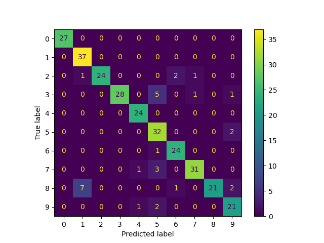
The handwritten digit dataset has 1797 total points. The model will be trained using all points, but only 30 will be labeled. Results in the form of a confusion matrix and a series of metrics over each class will be very good.

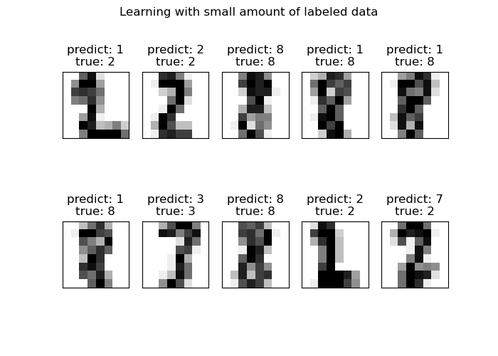
At the end, the top 10 most uncertain predictions will be shown.

# Authors: Clay Woolam <clay@woolam.org>
# License: BSD

Data generation

We use the digits dataset. We only use a subset of randomly selected samples.

import numpy as np

from sklearn import datasets

digits = datasets.load_digits()
rng = np.random.RandomState(2)
indices = np.arange(len(digits.data))
rng.shuffle(indices)

We selected 340 samples of which only 40 will be associated with a known label. Therefore, we store the indices of the 300 other samples for which we are not supposed to know their labels.

X = digits.data[indices[:340]]
y = digits.target[indices[:340]]
images = digits.images[indices[:340]]

n_total_samples = len(y)
n_labeled_points = 40

indices = np.arange(n_total_samples)

unlabeled_set = indices[n_labeled_points:]

Shuffle everything around

y_train = np.copy(y)
y_train[unlabeled_set] = -1

Semi-supervised learning

We fit a LabelSpreading and use it to predict the unknown labels.

from sklearn.metrics import classification_report
from sklearn.semi_supervised import LabelSpreading

lp_model = LabelSpreading(gamma=0.25, max_iter=20)
lp_model.fit(X, y_train)
predicted_labels = lp_model.transduction_[unlabeled_set]
true_labels = y[unlabeled_set]

print(
    "Label Spreading model: %d labeled & %d unlabeled points (%d total)"
    % (n_labeled_points, n_total_samples - n_labeled_points, n_total_samples)
)

Label Spreading model: 40 labeled & 300 unlabeled points (340 total)

Classification report

print(classification_report(true_labels, predicted_labels))

              precision    recall  f1-score   support

           0       1.00      1.00      1.00        27
           1       0.82      1.00      0.90        37
           2       1.00      0.86      0.92        28
           3       1.00      0.80      0.89        35
           4       0.92      1.00      0.96        24
           5       0.74      0.94      0.83        34
           6       0.89      0.96      0.92        25
           7       0.94      0.89      0.91        35
           8       1.00      0.68      0.81        31
           9       0.81      0.88      0.84        24

    accuracy                           0.90       300
   macro avg       0.91      0.90      0.90       300
weighted avg       0.91      0.90      0.90       300

Confusion matrix

from sklearn.metrics import ConfusionMatrixDisplay

ConfusionMatrixDisplay.from_predictions(
    true_labels, predicted_labels, labels=lp_model.classes_
)

<sklearn.metrics._plot.confusion_matrix.ConfusionMatrixDisplay object at 0x7f44c7ecdd30>

Plot the most uncertain predictions

Here, we will pick and show the 10 most uncertain predictions.

from scipy import stats

pred_entropies = stats.distributions.entropy(lp_model.label_distributions_.T)

Pick the top 10 most uncertain labels

uncertainty_index = np.argsort(pred_entropies)[-10:]

Plot

import matplotlib.pyplot as plt

f = plt.figure(figsize=(7, 5))
for index, image_index in enumerate(uncertainty_index):
    image = images[image_index]

    sub = f.add_subplot(2, 5, index + 1)
    sub.imshow(image, cmap=plt.cm.gray_r)
    plt.xticks([])
    plt.yticks([])
    sub.set_title(
        "predict: %i\ntrue: %i" % (lp_model.transduction_[image_index], y[image_index])
    )

f.suptitle("Learning with small amount of labeled data")
plt.show()