The Iris Dataset

This data sets consists of 3 different types of irises’ (Setosa, Versicolour, and Virginica) petal and sepal length, stored in a 150x4 numpy.ndarray

The rows being the samples and the columns being: Sepal Length, Sepal Width, Petal Length and Petal Width.

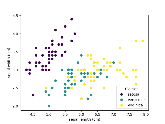
The below plot uses the first two features. See here for more information on this dataset.

# Code source: Gaël Varoquaux
# Modified for documentation by Jaques Grobler
# License: BSD 3 clause

Loading the iris dataset

from sklearn import datasets

iris = datasets.load_iris()

Scatter Plot of the Iris dataset

import matplotlib.pyplot as plt

_, ax = plt.subplots()
scatter = ax.scatter(iris.data[:, 0], iris.data[:, 1], c=iris.target)
ax.set(xlabel=iris.feature_names[0], ylabel=iris.feature_names[1])
_ = ax.legend(
    scatter.legend_elements()[0], iris.target_names, loc="lower right", title="Classes"
)

Each point in the scatter plot refers to one of the 150 iris flowers in the dataset, with the color indicating their respective type (Setosa, Versicolour, and Virginica). You can already see a pattern regarding the Setosa type, which is easily identifiable based on its short and wide sepal. Only considering these 2 dimensions, sepal width and length, there’s still overlap between the Versicolor and Virginica types.

Plot a PCA representation

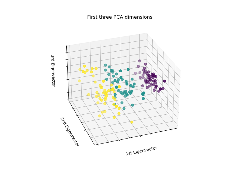
Let’s apply a Principal Component Analysis (PCA) to the iris dataset and then plot the irises across the first three PCA dimensions. This will allow us to better differentiate between the three types!

# unused but required import for doing 3d projections with matplotlib < 3.2
import mpl_toolkits.mplot3d  # noqa: F401

from sklearn.decomposition import PCA

fig = plt.figure(1, figsize=(8, 6))
ax = fig.add_subplot(111, projection="3d", elev=-150, azim=110)

X_reduced = PCA(n_components=3).fit_transform(iris.data)
ax.scatter(
    X_reduced[:, 0],
    X_reduced[:, 1],
    X_reduced[:, 2],
    c=iris.target,
    s=40,
)

ax.set_title("First three PCA dimensions")
ax.set_xlabel("1st Eigenvector")
ax.xaxis.set_ticklabels([])
ax.set_ylabel("2nd Eigenvector")
ax.yaxis.set_ticklabels([])
ax.set_zlabel("3rd Eigenvector")
ax.zaxis.set_ticklabels([])

plt.show()

PCA will create 3 new features that are a linear combination of the 4 original features. In addition, this transform maximizes the variance. With this transformation, we see that we can identify each species using only the first feature (i.e. first eigenvalues).