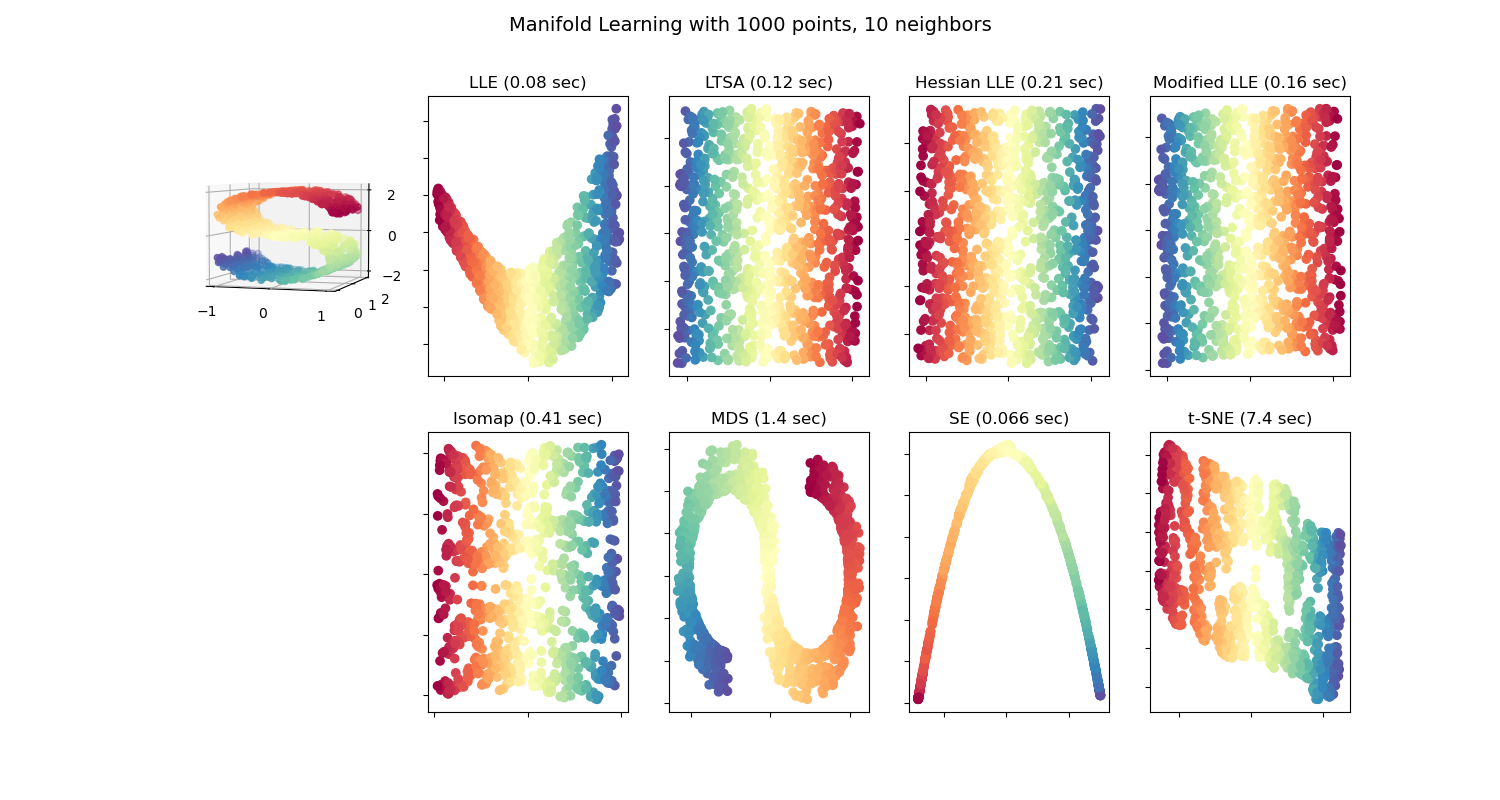
Comparison of Manifold Learning methods

An illustration of dimensionality reduction on the S-curve dataset with various manifold learning methods.

For a discussion and comparison of these algorithms, see the manifold module page

For a similar example, where the methods are applied to a sphere dataset, see Manifold Learning methods on a severed sphere

Note that the purpose of the MDS is to find a low-dimensional representation of the data (here 2D) in which the distances respect well the distances in the original high-dimensional space, unlike other manifold-learning algorithms, it does not seeks an isotropic representation of the data in the low-dimensional space.

Out:

LLE: 0.08 sec
LTSA: 0.12 sec
Hessian LLE: 0.21 sec
Modified LLE: 0.16 sec
Isomap: 0.41 sec
MDS: 1.4 sec
SE: 0.066 sec
/home/circleci/project/sklearn/manifold/_t_sne.py:790: FutureWarning: The default learning rate in TSNE will change from 200.0 to 'auto' in 1.2.
  warnings.warn(
/home/circleci/project/sklearn/manifold/_t_sne.py:982: FutureWarning: The PCA initialization in TSNE will change to have the standard deviation of PC1 equal to 1e-4 in 1.2. This will ensure better convergence.
  warnings.warn(
t-SNE: 7.4 sec

# Author: Jake Vanderplas -- <vanderplas@astro.washington.edu>

from collections import OrderedDict
from functools import partial
from time import time

import matplotlib.pyplot as plt
from mpl_toolkits.mplot3d import Axes3D
from matplotlib.ticker import NullFormatter

from sklearn import manifold, datasets

# Next line to silence pyflakes. This import is needed.
Axes3D

n_points = 1000
X, color = datasets.make_s_curve(n_points, random_state=0)
n_neighbors = 10
n_components = 2

# Create figure
fig = plt.figure(figsize=(15, 8))
fig.suptitle(
    "Manifold Learning with %i points, %i neighbors" % (1000, n_neighbors), fontsize=14
)

# Add 3d scatter plot
ax = fig.add_subplot(251, projection="3d")
ax.scatter(X[:, 0], X[:, 1], X[:, 2], c=color, cmap=plt.cm.Spectral)
ax.view_init(4, -72)

# Set-up manifold methods
LLE = partial(
    manifold.LocallyLinearEmbedding,
    n_neighbors=n_neighbors,
    n_components=n_components,
    eigen_solver="auto",
)

methods = OrderedDict()
methods["LLE"] = LLE(method="standard")
methods["LTSA"] = LLE(method="ltsa")
methods["Hessian LLE"] = LLE(method="hessian")
methods["Modified LLE"] = LLE(method="modified")
methods["Isomap"] = manifold.Isomap(n_neighbors=n_neighbors, n_components=n_components)
methods["MDS"] = manifold.MDS(n_components, max_iter=100, n_init=1)
methods["SE"] = manifold.SpectralEmbedding(
    n_components=n_components, n_neighbors=n_neighbors
)
methods["t-SNE"] = manifold.TSNE(n_components=n_components, init="pca", random_state=0)

# Plot results
for i, (label, method) in enumerate(methods.items()):
    t0 = time()
    Y = method.fit_transform(X)
    t1 = time()
    print("%s: %.2g sec" % (label, t1 - t0))
    ax = fig.add_subplot(2, 5, 2 + i + (i > 3))
    ax.scatter(Y[:, 0], Y[:, 1], c=color, cmap=plt.cm.Spectral)
    ax.set_title("%s (%.2g sec)" % (label, t1 - t0))
    ax.xaxis.set_major_formatter(NullFormatter())
    ax.yaxis.set_major_formatter(NullFormatter())
    ax.axis("tight")

plt.show()