Illustration of prior and posterior Gaussian process for different kernels

This example illustrates the prior and posterior of a GaussianProcessRegressor with different kernels. Mean, standard deviation, and 5 samples are shown for both prior and posterior distributions.

Here, we only give some illustration. To know more about kernels’ formulation, refer to the User Guide.

# Authors: Jan Hendrik Metzen <jhm@informatik.uni-bremen.de>
#          Guillaume Lemaitre <g.lemaitre58@gmail.com>
# License: BSD 3 clause

Helper function

Before presenting each individual kernel available for Gaussian processes, we will define an helper function allowing us plotting samples drawn from the Gaussian process.

This function will take a GaussianProcessRegressor model and will drawn sample from the Gaussian process. If the model was not fit, the samples are drawn from the prior distribution while after model fitting, the samples are drawn from the posterior distribution.

import matplotlib.pyplot as plt
import numpy as np


def plot_gpr_samples(gpr_model, n_samples, ax):
    """Plot samples drawn from the Gaussian process model.

    If the Gaussian process model is not trained then the drawn samples are
    drawn from the prior distribution. Otherwise, the samples are drawn from
    the posterior distribution. Be aware that a sample here corresponds to a
    function.

    Parameters
    ----------
    gpr_model : `GaussianProcessRegressor`
        A :class:`~sklearn.gaussian_process.GaussianProcessRegressor` model.
    n_samples : int
        The number of samples to draw from the Gaussian process distribution.
    ax : matplotlib axis
        The matplotlib axis where to plot the samples.
    """
    x = np.linspace(0, 5, 100)
    X = x.reshape(-1, 1)

    y_mean, y_std = gpr_model.predict(X, return_std=True)
    y_samples = gpr_model.sample_y(X, n_samples)

    for idx, single_prior in enumerate(y_samples.T):
        ax.plot(
            x,
            single_prior,
            linestyle="--",
            alpha=0.7,
            label=f"Sampled function #{idx + 1}",
        )
    ax.plot(x, y_mean, color="black", label="Mean")
    ax.fill_between(
        x,
        y_mean - y_std,
        y_mean + y_std,
        alpha=0.1,
        color="black",
        label=r"$\pm$ 1 std. dev.",
    )
    ax.set_xlabel("x")
    ax.set_ylabel("y")
    ax.set_ylim([-3, 3])

Dataset and Gaussian process generation

We will create a training dataset that we will use in the different sections.

rng = np.random.RandomState(4)
X_train = rng.uniform(0, 5, 10).reshape(-1, 1)
y_train = np.sin((X_train[:, 0] - 2.5) ** 2)
n_samples = 5

Kernel cookbook

In this section, we illustrate some samples drawn from the prior and posterior distributions of the Gaussian process with different kernels.

Radial Basis Function kernel

from sklearn.gaussian_process import GaussianProcessRegressor
from sklearn.gaussian_process.kernels import RBF

kernel = 1.0 * RBF(length_scale=1.0, length_scale_bounds=(1e-1, 10.0))
gpr = GaussianProcessRegressor(kernel=kernel, random_state=0)

fig, axs = plt.subplots(nrows=2, sharex=True, sharey=True, figsize=(10, 8))

# plot prior
plot_gpr_samples(gpr, n_samples=n_samples, ax=axs[0])
axs[0].set_title("Samples from prior distribution")

# plot posterior
gpr.fit(X_train, y_train)
plot_gpr_samples(gpr, n_samples=n_samples, ax=axs[1])
axs[1].scatter(X_train[:, 0], y_train, color="red", zorder=10, label="Observations")
axs[1].legend(bbox_to_anchor=(1.05, 1.5), loc="upper left")
axs[1].set_title("Samples from posterior distribution")

fig.suptitle("Radial Basis Function kernel", fontsize=18)
plt.tight_layout()

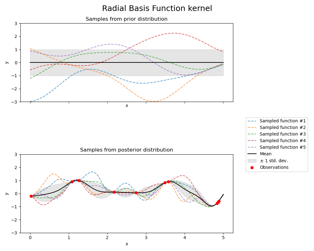
print(f"Kernel parameters before fit:\n{kernel})")
print(
    f"Kernel parameters after fit: \n{gpr.kernel_} \n"
    f"Log-likelihood: {gpr.log_marginal_likelihood(gpr.kernel_.theta):.3f}"
)

Out:

Kernel parameters before fit:
1**2 * RBF(length_scale=1))
Kernel parameters after fit:
0.594**2 * RBF(length_scale=0.279)
Log-likelihood: -0.067

Rational Quadradtic kernel

from sklearn.gaussian_process.kernels import RationalQuadratic

kernel = 1.0 * RationalQuadratic(length_scale=1.0, alpha=0.1, alpha_bounds=(1e-5, 1e15))
gpr = GaussianProcessRegressor(kernel=kernel, random_state=0)

fig, axs = plt.subplots(nrows=2, sharex=True, sharey=True, figsize=(10, 8))

# plot prior
plot_gpr_samples(gpr, n_samples=n_samples, ax=axs[0])
axs[0].set_title("Samples from prior distribution")

# plot posterior
gpr.fit(X_train, y_train)
plot_gpr_samples(gpr, n_samples=n_samples, ax=axs[1])
axs[1].scatter(X_train[:, 0], y_train, color="red", zorder=10, label="Observations")
axs[1].legend(bbox_to_anchor=(1.05, 1.5), loc="upper left")
axs[1].set_title("Samples from posterior distribution")

fig.suptitle("Rational Quadratic kernel", fontsize=18)
plt.tight_layout()

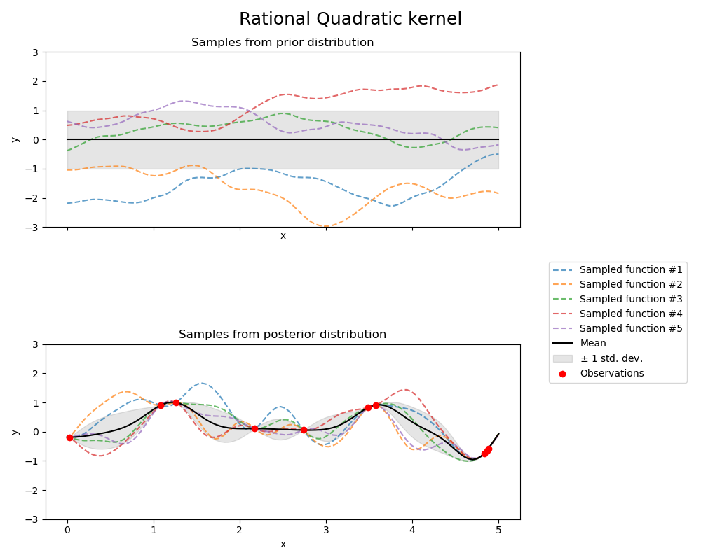
print(f"Kernel parameters before fit:\n{kernel})")
print(
    f"Kernel parameters after fit: \n{gpr.kernel_} \n"
    f"Log-likelihood: {gpr.log_marginal_likelihood(gpr.kernel_.theta):.3f}"
)

Out:

Kernel parameters before fit:
1**2 * RationalQuadratic(alpha=0.1, length_scale=1))
Kernel parameters after fit:
0.594**2 * RationalQuadratic(alpha=8.5e+05, length_scale=0.279)
Log-likelihood: -0.067

Periodic kernel

from sklearn.gaussian_process.kernels import ExpSineSquared

kernel = 1.0 * ExpSineSquared(
    length_scale=1.0,
    periodicity=3.0,
    length_scale_bounds=(0.1, 10.0),
    periodicity_bounds=(1.0, 10.0),
)
gpr = GaussianProcessRegressor(kernel=kernel, random_state=0)

fig, axs = plt.subplots(nrows=2, sharex=True, sharey=True, figsize=(10, 8))

# plot prior
plot_gpr_samples(gpr, n_samples=n_samples, ax=axs[0])
axs[0].set_title("Samples from prior distribution")

# plot posterior
gpr.fit(X_train, y_train)
plot_gpr_samples(gpr, n_samples=n_samples, ax=axs[1])
axs[1].scatter(X_train[:, 0], y_train, color="red", zorder=10, label="Observations")
axs[1].legend(bbox_to_anchor=(1.05, 1.5), loc="upper left")
axs[1].set_title("Samples from posterior distribution")

fig.suptitle("Periodic kernel", fontsize=18)
plt.tight_layout()

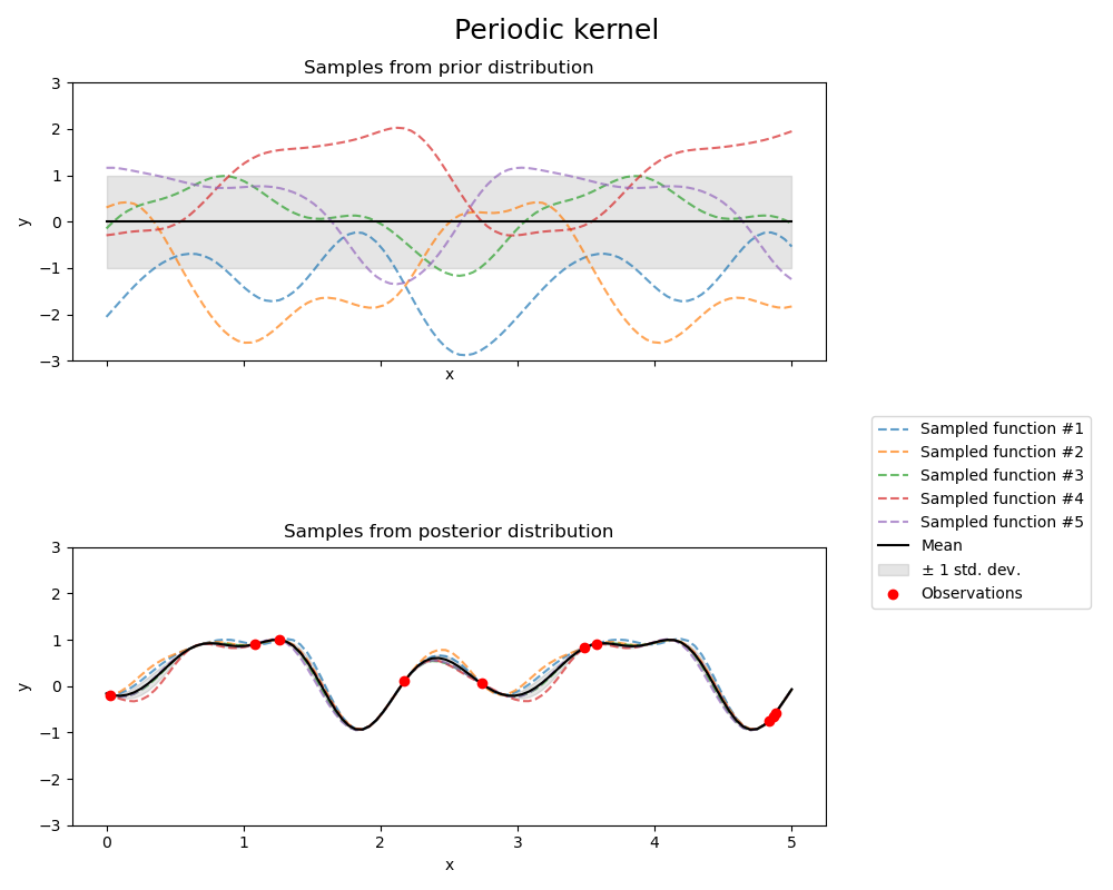
print(f"Kernel parameters before fit:\n{kernel})")
print(
    f"Kernel parameters after fit: \n{gpr.kernel_} \n"
    f"Log-likelihood: {gpr.log_marginal_likelihood(gpr.kernel_.theta):.3f}"
)

Out:

Kernel parameters before fit:
1**2 * ExpSineSquared(length_scale=1, periodicity=3))
Kernel parameters after fit:
0.799**2 * ExpSineSquared(length_scale=0.791, periodicity=2.87)
Log-likelihood: 3.394

Dot product kernel

from sklearn.gaussian_process.kernels import ConstantKernel, DotProduct

kernel = ConstantKernel(0.1, (0.01, 10.0)) * (
    DotProduct(sigma_0=1.0, sigma_0_bounds=(0.1, 10.0)) ** 2
)
gpr = GaussianProcessRegressor(kernel=kernel, random_state=0)

fig, axs = plt.subplots(nrows=2, sharex=True, sharey=True, figsize=(10, 8))

# plot prior
plot_gpr_samples(gpr, n_samples=n_samples, ax=axs[0])
axs[0].set_title("Samples from prior distribution")

# plot posterior
gpr.fit(X_train, y_train)
plot_gpr_samples(gpr, n_samples=n_samples, ax=axs[1])
axs[1].scatter(X_train[:, 0], y_train, color="red", zorder=10, label="Observations")
axs[1].legend(bbox_to_anchor=(1.05, 1.5), loc="upper left")
axs[1].set_title("Samples from posterior distribution")

fig.suptitle("Dot product kernel", fontsize=18)
plt.tight_layout()

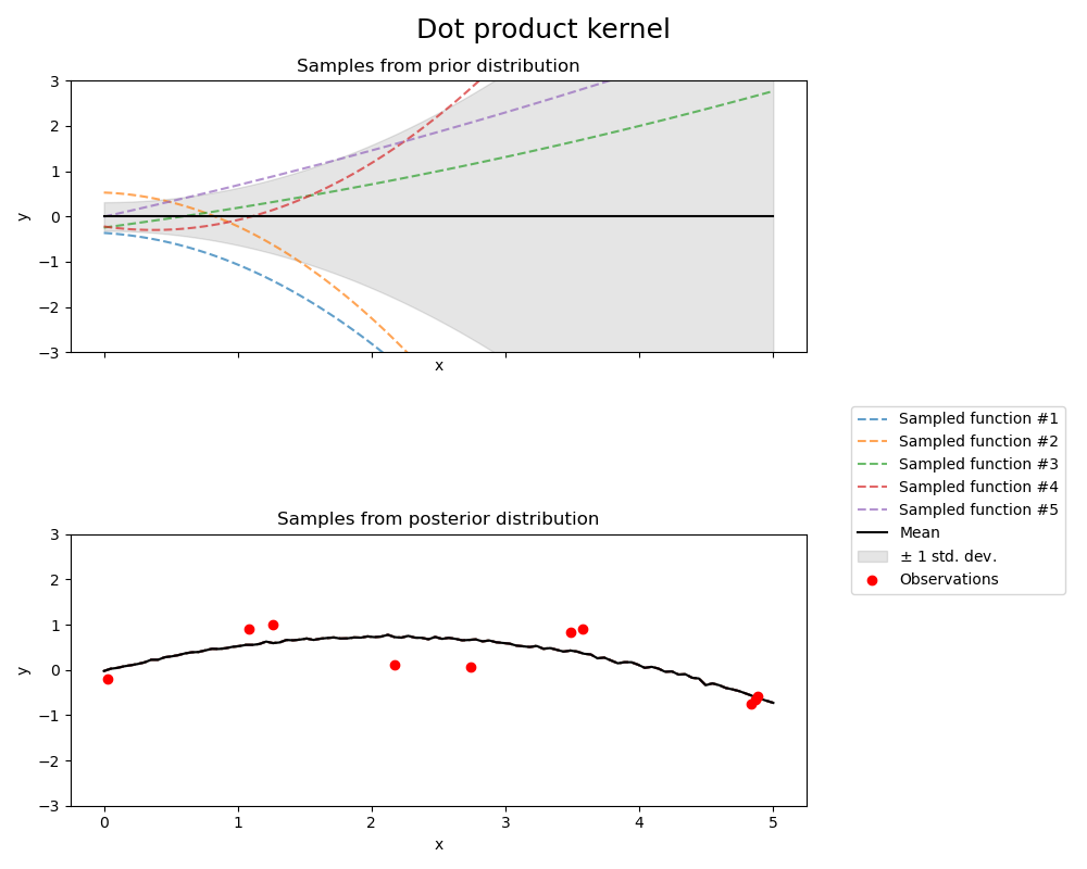
Out:

/home/circleci/project/sklearn/gaussian_process/kernels.py:430: ConvergenceWarning: The optimal value found for dimension 0 of parameter k1__constant_value is close to the specified upper bound 10.0. Increasing the bound and calling fit again may find a better value.
  warnings.warn(

print(f"Kernel parameters before fit:\n{kernel})")
print(
    f"Kernel parameters after fit: \n{gpr.kernel_} \n"
    f"Log-likelihood: {gpr.log_marginal_likelihood(gpr.kernel_.theta):.3f}"
)

Out:

Kernel parameters before fit:
0.316**2 * DotProduct(sigma_0=1) ** 2)
Kernel parameters after fit:
3.16**2 * DotProduct(sigma_0=5.26) ** 2
Log-likelihood: -7708734861.459

Mattern kernel

from sklearn.gaussian_process.kernels import Matern

kernel = 1.0 * Matern(length_scale=1.0, length_scale_bounds=(1e-1, 10.0), nu=1.5)
gpr = GaussianProcessRegressor(kernel=kernel, random_state=0)

fig, axs = plt.subplots(nrows=2, sharex=True, sharey=True, figsize=(10, 8))

# plot prior
plot_gpr_samples(gpr, n_samples=n_samples, ax=axs[0])
axs[0].set_title("Samples from prior distribution")

# plot posterior
gpr.fit(X_train, y_train)
plot_gpr_samples(gpr, n_samples=n_samples, ax=axs[1])
axs[1].scatter(X_train[:, 0], y_train, color="red", zorder=10, label="Observations")
axs[1].legend(bbox_to_anchor=(1.05, 1.5), loc="upper left")
axs[1].set_title("Samples from posterior distribution")

fig.suptitle("Mattern kernel", fontsize=18)
plt.tight_layout()

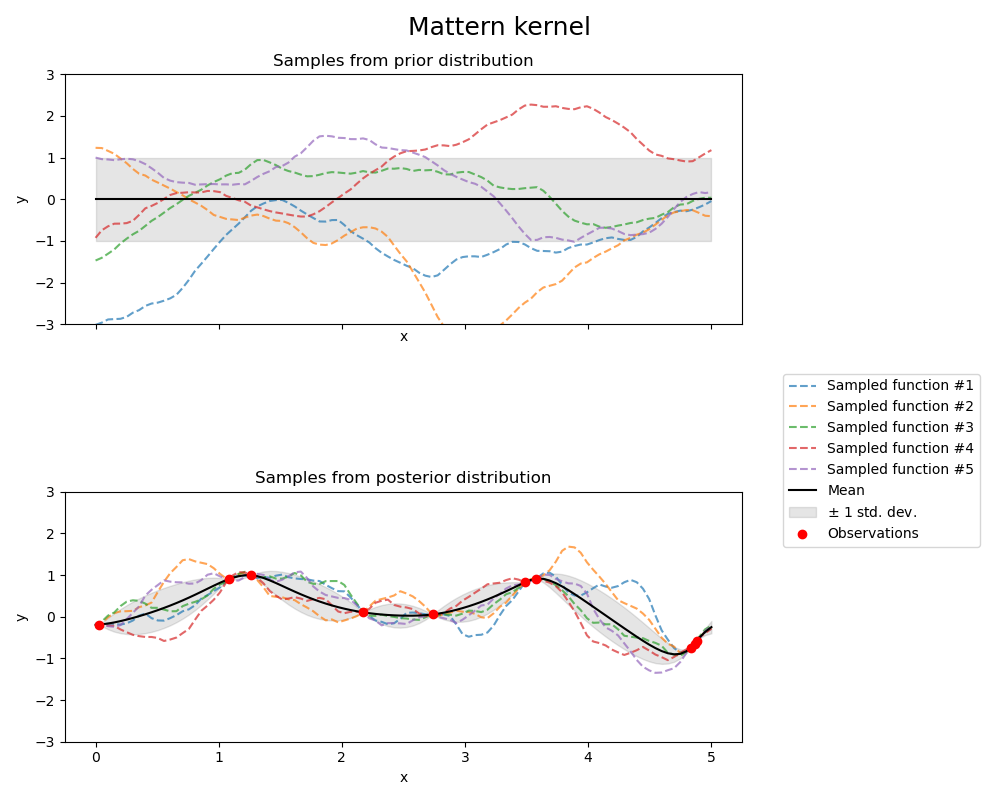
print(f"Kernel parameters before fit:\n{kernel})")
print(
    f"Kernel parameters after fit: \n{gpr.kernel_} \n"
    f"Log-likelihood: {gpr.log_marginal_likelihood(gpr.kernel_.theta):.3f}"
)

Out:

Kernel parameters before fit:
1**2 * Matern(length_scale=1, nu=1.5))
Kernel parameters after fit:
0.609**2 * Matern(length_scale=0.484, nu=1.5)
Log-likelihood: -1.185