Note
Click here to download the full example code or to run this example in your browser via Binder
Principal Component Regression vs Partial Least Squares Regression
This example compares Principal Component Regression (PCR) and Partial Least Squares Regression (PLS) on a toy dataset. Our goal is to illustrate how PLS can outperform PCR when the target is strongly correlated with some directions in the data that have a low variance.
PCR is a regressor composed of two steps: first,
PCA is applied to the training data, possibly
performing dimensionality reduction; then, a regressor (e.g. a linear
regressor) is trained on the transformed samples. In
PCA, the transformation is purely
unsupervised, meaning that no information about the targets is used. As a
result, PCR may perform poorly in some datasets where the target is strongly
correlated with directions that have low variance. Indeed, the
dimensionality reduction of PCA projects the data into a lower dimensional
space where the variance of the projected data is greedily maximized along
each axis. Despite them having the most predictive power on the target, the
directions with a lower variance will be dropped, and the final regressor
will not be able to leverage them.
PLS is both a transformer and a regressor, and it is quite similar to PCR: it also applies a dimensionality reduction to the samples before applying a linear regressor to the transformed data. The main difference with PCR is that the PLS transformation is supervised. Therefore, as we will see in this example, it does not suffer from the issue we just mentioned.
The data
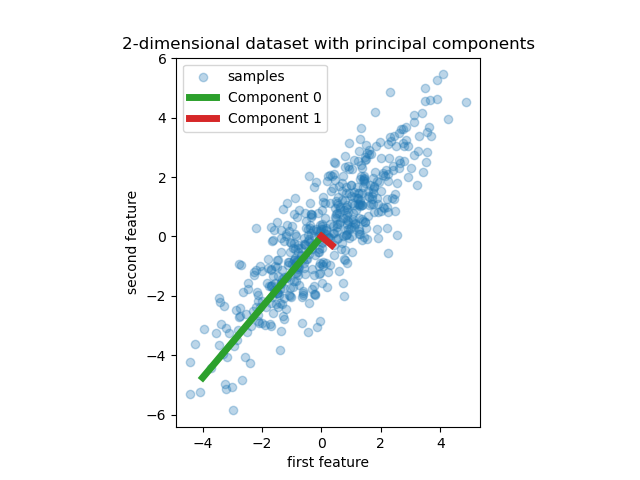
We start by creating a simple dataset with two features. Before we even dive into PCR and PLS, we fit a PCA estimator to display the two principal components of this dataset, i.e. the two directions that explain the most variance in the data.
import numpy as np
import matplotlib.pyplot as plt
from sklearn.decomposition import PCA

rng = np.random.RandomState(0)
n_samples = 500
cov = [[3, 3], [3, 4]]
X = rng.multivariate_normal(mean=[0, 0], cov=cov, size=n_samples)
pca = PCA(n_components=2).fit(X)


plt.scatter(X[:, 0], X[:, 1], alpha=0.3, label="samples")
for i, (comp, var) in enumerate(zip(pca.components_, pca.explained_variance_)):
    comp = comp * var  # scale component by its variance explanation power
    plt.plot(
        [0, comp[0]],
        [0, comp[1]],
        label=f"Component {i}",
        linewidth=5,
        color=f"C{i + 2}",
    )
plt.gca().set(
    aspect="equal",
    title="2-dimensional dataset with principal components",
    xlabel="first feature",
    ylabel="second feature",
)
plt.legend()
plt.show()
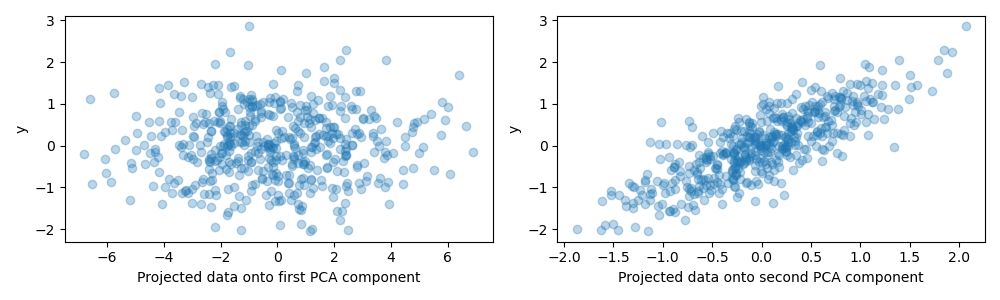
For the purpose of this example, we now define the target y such that it is
strongly correlated with a direction that has a small variance. To this end,
we will project X onto the second component, and add some noise to it.
y = X.dot(pca.components_[1]) + rng.normal(size=n_samples) / 2

fig, axes = plt.subplots(1, 2, figsize=(10, 3))

axes[0].scatter(X.dot(pca.components_[0]), y, alpha=0.3)
axes[0].set(xlabel="Projected data onto first PCA component", ylabel="y")
axes[1].scatter(X.dot(pca.components_[1]), y, alpha=0.3)
axes[1].set(xlabel="Projected data onto second PCA component", ylabel="y")
plt.tight_layout()
plt.show()
Projection on one component and predictive power
We now create two regressors: PCR and PLS, and for our illustration purposes we set the number of components to 1. Before feeding the data to the PCA step of PCR, we first standardize it, as recommended by good practice. The PLS estimator has built-in scaling capabilities.
For both models, we plot the projected data onto the first component against the target. In both cases, this projected data is what the regressors will use as training data.
from sklearn.model_selection import train_test_split
from sklearn.pipeline import make_pipeline
from sklearn.linear_model import LinearRegression
from sklearn.preprocessing import StandardScaler
from sklearn.decomposition import PCA
from sklearn.cross_decomposition import PLSRegression

X_train, X_test, y_train, y_test = train_test_split(X, y, random_state=rng)

pcr = make_pipeline(StandardScaler(), PCA(n_components=1), LinearRegression())
pcr.fit(X_train, y_train)
pca = pcr.named_steps["pca"]  # retrieve the PCA step of the pipeline

pls = PLSRegression(n_components=1)
pls.fit(X_train, y_train)

fig, axes = plt.subplots(1, 2, figsize=(10, 3))
axes[0].scatter(pca.transform(X_test), y_test, alpha=0.3, label="ground truth")
axes[0].scatter(
    pca.transform(X_test), pcr.predict(X_test), alpha=0.3, label="predictions"
)
axes[0].set(
    xlabel="Projected data onto first PCA component", ylabel="y", title="PCR / PCA"
)
axes[0].legend()
axes[1].scatter(pls.transform(X_test), y_test, alpha=0.3, label="ground truth")
axes[1].scatter(
    pls.transform(X_test), pls.predict(X_test), alpha=0.3, label="predictions"
)
axes[1].set(xlabel="Projected data onto first PLS component", ylabel="y", title="PLS")
axes[1].legend()
plt.tight_layout()
plt.show()
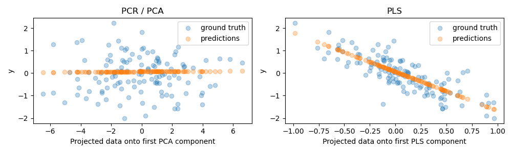
As expected, the unsupervised PCA transformation of PCR has dropped the second component, i.e. the direction with the lowest variance, despite it being the most predictive direction. This is because PCA is a completely unsupervised transformation, and results in the projected data having a low predictive power on the target.
On the other hand, the PLS regressor manages to capture the effect of the direction with the lowest variance, thanks to its use of target information during the transformation: it can recognize that this direction is actually the most predictive. We note that the first PLS component is negatively correlated with the target, which comes from the fact that the signs of eigenvectors are arbitrary.
We also print the R-squared scores of both estimators, which further confirms that PLS is a better alternative than PCR in this case. A negative R-squared indicates that PCR performs worse than a regressor that would simply predict the mean of the target.
print(f"PCR r-squared {pcr.score(X_test, y_test):.3f}")
print(f"PLS r-squared {pls.score(X_test, y_test):.3f}")
Out:
PCR r-squared -0.026
PLS r-squared 0.658
As a final remark, we note that PCR with 2 components performs as well as PLS: this is because in this case, PCR was able to leverage the second component which has the most preditive power on the target.
pca_2 = make_pipeline(PCA(n_components=2), LinearRegression())
pca_2.fit(X_train, y_train)
print(f"PCR r-squared with 2 components {pca_2.score(X_test, y_test):.3f}")
Out:
PCR r-squared with 2 components 0.673
Total running time of the script: ( 0 minutes 0.368 seconds)