1.16. Probability calibration¶

1.16.1. Calibration curves¶

The following plot compares how well the probabilistic predictions of different classifiers are calibrated, using calibration_curve. The x axis represents the average predicted probability in each bin. The y axis is the fraction of positives, i.e. the proportion of samples whose class is the positive class (in each bin).

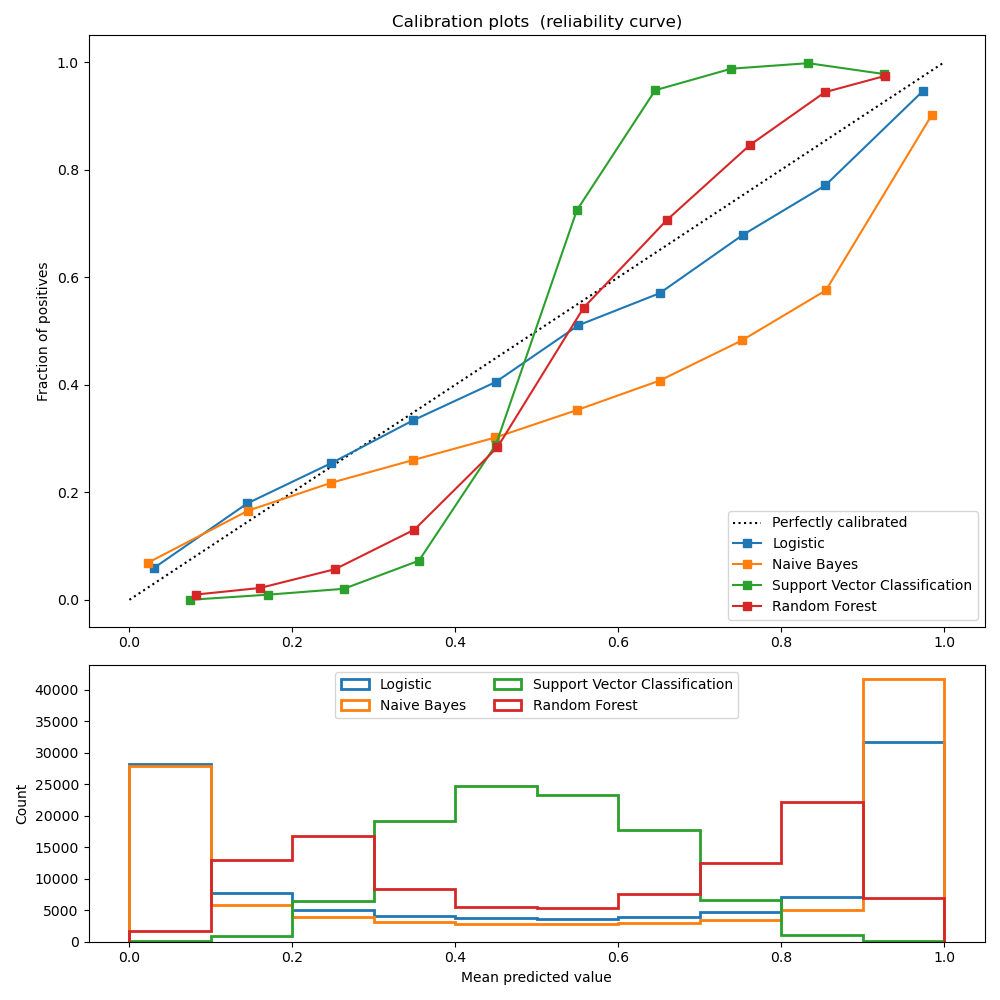
LogisticRegression returns well calibrated predictions by default as it directly optimizes log-loss. In contrast, the other methods return biased probabilities; with different biases per method:

GaussianNB tends to push probabilities to 0 or 1 (note the counts in the histograms). This is mainly because it makes the assumption that features are conditionally independent given the class, which is not the case in this dataset which contains 2 redundant features.

RandomForestClassifier shows the opposite behavior: the histograms show peaks at approximately 0.2 and 0.9 probability, while probabilities close to 0 or 1 are very rare. An explanation for this is given by Niculescu-Mizil and Caruana 1: “Methods such as bagging and random forests that average predictions from a base set of models can have difficulty making predictions near 0 and 1 because variance in the underlying base models will bias predictions that should be near zero or one away from these values. Because predictions are restricted to the interval [0,1], errors caused by variance tend to be one-sided near zero and one. For example, if a model should predict p = 0 for a case, the only way bagging can achieve this is if all bagged trees predict zero. If we add noise to the trees that bagging is averaging over, this noise will cause some trees to predict values larger than 0 for this case, thus moving the average prediction of the bagged ensemble away from 0. We observe this effect most strongly with random forests because the base-level trees trained with random forests have relatively high variance due to feature subsetting.” As a result, the calibration curve also referred to as the reliability diagram (Wilks 1995 2) shows a characteristic sigmoid shape, indicating that the classifier could trust its “intuition” more and return probabilities closer to 0 or 1 typically.

Linear Support Vector Classification (LinearSVC) shows an even more sigmoid curve as the RandomForestClassifier, which is typical for maximum-margin methods (compare Niculescu-Mizil and Caruana 1), which focus on hard samples that are close to the decision boundary (the support vectors).

1.16.2. Calibrating a classifier¶

Calibrating a classifier consists in fitting a regressor (called a calibrator) that maps the output of the classifier (as given by predict or predict_proba) to a calibrated probability in [0, 1]. Denoting the output of the classifier for a given sample by \(f_i\), the calibrator tries to predict \(p(y_i = 1 | f_i)\).

The samples that are used to train the calibrator should not be used to train the target classifier.

1.16.3. Usage¶

The CalibratedClassifierCV class is used to calibrate a classifier.

CalibratedClassifierCV uses a cross-validation approach to fit both the classifier and the regressor. For each of the k (trainset, testset) couple, a classifier is trained on the train set, and its predictions on the test set are used to fit a regressor. We end up with k (classifier, regressor) couples where each regressor maps the output of its corresponding classifier into [0, 1]. Each couple is exposed in the calibrated_classifiers_ attribute, where each entry is a calibrated classifier with a predict_proba method that outputs calibrated probabilities. The output of predict_proba for the main CalibratedClassifierCV instance corresponds to the average of the predicted probabilities of the k estimators in the calibrated_classifiers_ list. The output of predict is the class that has the highest probability.

The regressor that is used for calibration depends on the method parameter. 'sigmoid' corresponds to a parametric approach based on Platt’s logistic model 3, i.e. \(p(y_i = 1 | f_i)\) is modeled as \(\sigma(A f_i + B)\) where \(\sigma\) is the logistic function, and \(A\) and \(B\) are real numbers to be determined when fitting the regressor via maximum likelihood. 'isotonic' will instead fit a non-parametric isotonic regressor, which outputs a step-wise non-decreasing function (see sklearn.isotonic).

An already fitted classifier can be calibrated by setting cv="prefit". In this case, the data is only used to fit the regressor. It is up to the user make sure that the data used for fitting the classifier is disjoint from the data used for fitting the regressor.

CalibratedClassifierCV can calibrate probabilities in a multiclass setting if the base estimator supports multiclass predictions. The classifier is calibrated first for each class separately in a one-vs-rest fashion 4. When predicting probabilities, the calibrated probabilities for each class are predicted separately. As those probabilities do not necessarily sum to one, a postprocessing is performed to normalize them.

The sklearn.metrics.brier_score_loss may be used to evaluate how well a classifier is calibrated.

References:

- 1(1,2)
Predicting Good Probabilities with Supervised Learning, A. Niculescu-Mizil & R. Caruana, ICML 2005
- 2
On the combination of forecast probabilities for consecutive precipitation periods. Wea. Forecasting, 5, 640–650., Wilks, D. S., 1990a
- 3
Probabilistic Outputs for Support Vector Machines and Comparisons to Regularized Likelihood Methods, J. Platt, (1999)
- 4
Transforming Classifier Scores into Accurate Multiclass Probability Estimates, B. Zadrozny & C. Elkan, (KDD 2002)