Note

Click here to download the full example code or to run this example in your browser via Binder

Advanced Plotting With Partial Dependence¶

The plot_partial_dependence function returns a PartialDependenceDisplay object that can be used for plotting without needing to recalculate the partial dependence. In this example, we show how to plot partial dependence plots and how to quickly customize the plot with the visualization API.

Note

print(__doc__)

import pandas as pd
import matplotlib.pyplot as plt
from sklearn.datasets import load_diabetes
from sklearn.neural_network import MLPRegressor
from sklearn.preprocessing import StandardScaler
from sklearn.pipeline import make_pipeline
from sklearn.tree import DecisionTreeRegressor
from sklearn.inspection import plot_partial_dependence

Train models on the diabetes dataset¶

First, we train a decision tree and a multi-layer perceptron on the diabetes dataset.

diabetes = load_diabetes()
X = pd.DataFrame(diabetes.data, columns=diabetes.feature_names)
y = diabetes.target

tree = DecisionTreeRegressor()
mlp = make_pipeline(StandardScaler(),
                    MLPRegressor(hidden_layer_sizes=(100, 100),
                                 tol=1e-2, max_iter=500, random_state=0))
tree.fit(X, y)
mlp.fit(X, y)

Pipeline

Pipeline(steps=[('standardscaler', StandardScaler()),
                ('mlpregressor',
                 MLPRegressor(hidden_layer_sizes=(100, 100), max_iter=500,
                              random_state=0, tol=0.01))])

StandardScaler

StandardScaler()

MLPRegressor

MLPRegressor(hidden_layer_sizes=(100, 100), max_iter=500, random_state=0,
             tol=0.01)

Plotting partial dependence for two features¶

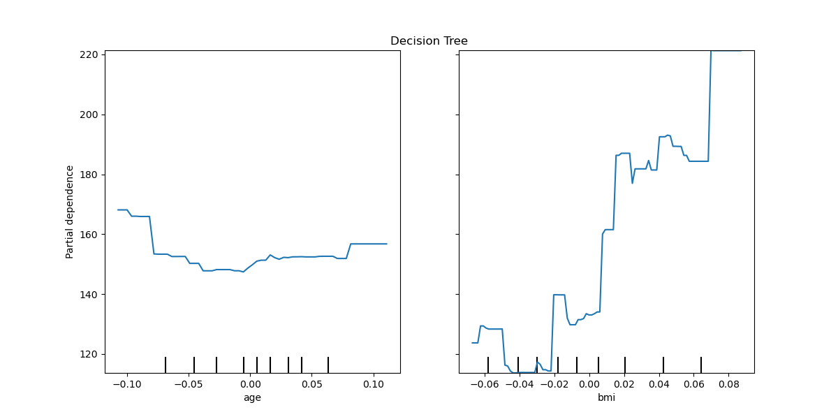
We plot partial dependence curves for features “age” and “bmi” (body mass index) for the decision tree. With two features, plot_partial_dependence expects to plot two curves. Here the plot function place a grid of two plots using the space defined by ax .

fig, ax = plt.subplots(figsize=(12, 6))
ax.set_title("Decision Tree")
tree_disp = plot_partial_dependence(tree, X, ["age", "bmi"], ax=ax)

Out:

/home/circleci/project/sklearn/tree/_classes.py:1254: FutureWarning: the classes_ attribute is to be deprecated from version 0.22 and will be removed in 0.24.
  warnings.warn(msg, FutureWarning)

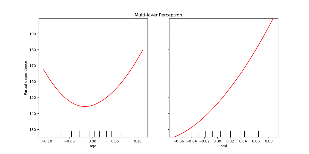
The partial depdendence curves can be plotted for the multi-layer perceptron. In this case, line_kw is passed to plot_partial_dependence to change the color of the curve.

fig, ax = plt.subplots(figsize=(12, 6))
ax.set_title("Multi-layer Perceptron")
mlp_disp = plot_partial_dependence(mlp, X, ["age", "bmi"], ax=ax,
                                   line_kw={"c": "red"})

Plotting partial dependence of the two models together¶

The tree_disp and mlp_disp PartialDependenceDisplay objects contain all the computed information needed to recreate the partial dependence curves. This means we can easily create additional plots without needing to recompute the curves.

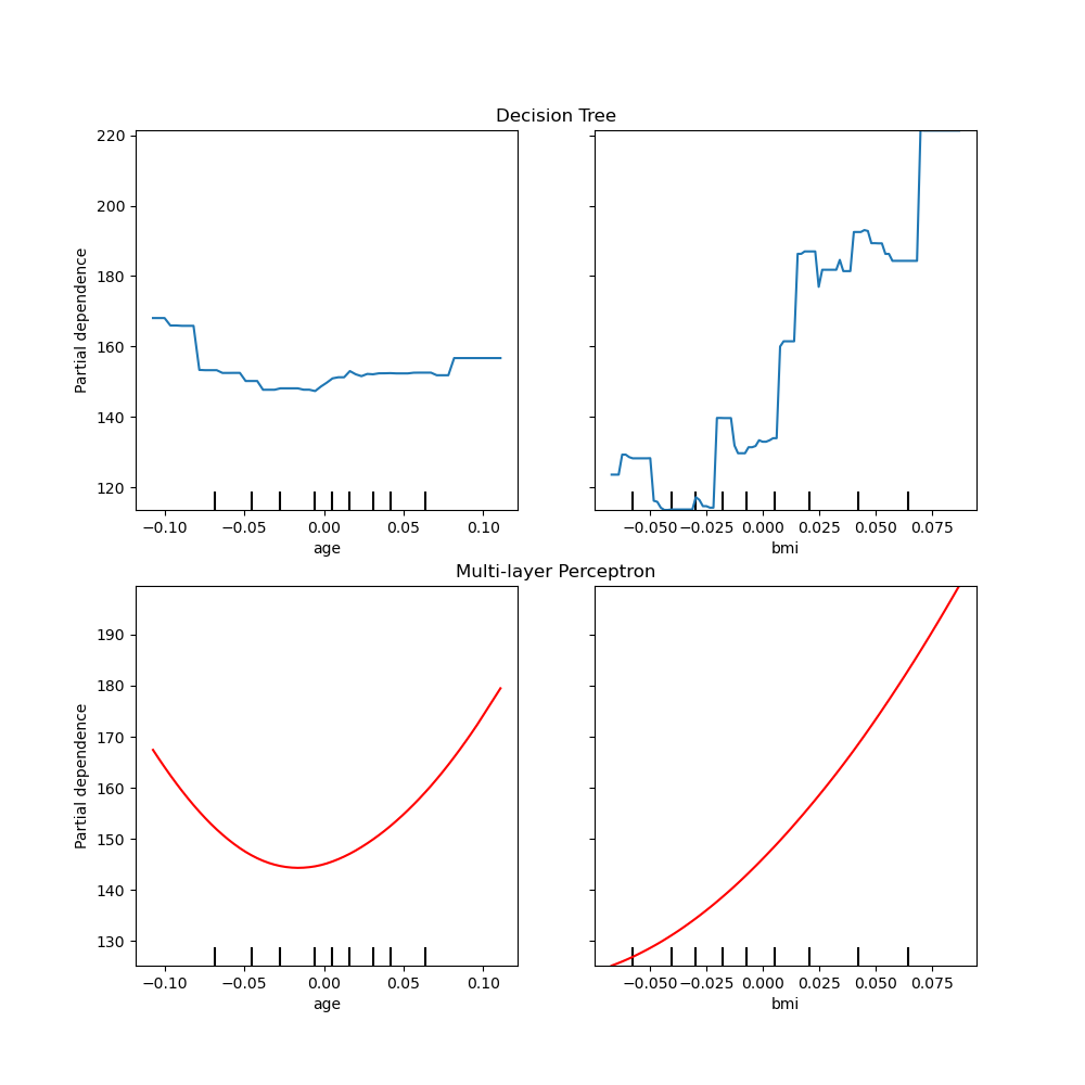
One way to plot the curves is to place them in the same figure, with the curves of each model on each row. First, we create a figure with two axes within two rows and one column. The two axes are passed to the plot functions of tree_disp and mlp_disp. The given axes will be used by the plotting function to draw the partial dependence. The resulting plot places the decision tree partial dependence curves in the first row of the multi-layer perceptron in the second row.

fig, (ax1, ax2) = plt.subplots(2, 1, figsize=(10, 10))
tree_disp.plot(ax=ax1)
ax1.set_title("Decision Tree")
mlp_disp.plot(ax=ax2, line_kw={"c": "red"})
ax2.set_title("Multi-layer Perceptron")

Out:

Text(0.5, 1.0, 'Multi-layer Perceptron')

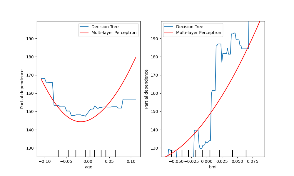
Another way to compare the curves is to plot them on top of each other. Here, we create a figure with one row and two columns. The axes are passed into the plot function as a list, which will plot the partial dependence curves of each model on the same axes. The length of the axes list must be equal to the number of plots drawn.

fig, (ax1, ax2) = plt.subplots(1, 2, figsize=(10, 6))
tree_disp.plot(ax=[ax1, ax2], line_kw={"label": "Decision Tree"})
mlp_disp.plot(ax=[ax1, ax2], line_kw={"label": "Multi-layer Perceptron",
                                      "c": "red"})
ax1.legend()
ax2.legend()

plot partial dependence visualization api

Out:

<matplotlib.legend.Legend object at 0x7f6357c3ad00>

tree_disp.axes_ is a numpy array container the axes used to draw the partial dependence plots. This can be passed to mlp_disp to have the same affect of drawing the plots on top of each other. Furthermore, the mlp_disp.figure_ stores the figure, which allows for resizing the figure after calling plot. In this case tree_disp.axes_ has two dimensions, thus plot will only show the y label and y ticks on the left most plot.

tree_disp.plot(line_kw={"label": "Decision Tree"})
mlp_disp.plot(line_kw={"label": "Multi-layer Perceptron", "c": "red"},
              ax=tree_disp.axes_)
tree_disp.figure_.set_size_inches(10, 6)
tree_disp.axes_[0, 0].legend()
tree_disp.axes_[0, 1].legend()
plt.show()

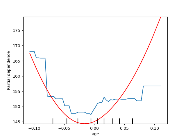
Plotting partial dependence for one feature¶

Here, we plot the partial dependence curves for a single feature, “age”, on the same axes. In this case, tree_disp.axes_ is passed into the second plot function.

tree_disp = plot_partial_dependence(tree, X, ["age"])
mlp_disp = plot_partial_dependence(mlp, X, ["age"],
                                   ax=tree_disp.axes_, line_kw={"c": "red"})

Out:

/home/circleci/project/sklearn/tree/_classes.py:1254: FutureWarning: the classes_ attribute is to be deprecated from version 0.22 and will be removed in 0.24.
  warnings.warn(msg, FutureWarning)

Total running time of the script: ( 0 minutes 2.971 seconds)

Gallery generated by Sphinx-Gallery