
1.16. Probability calibration
When performing classification you often want not only to predict the class label, but also obtain a probability of the respective label. This probability gives you some kind of confidence on the prediction. Some models can give you poor estimates of the class probabilities and some even do not support probability prediction. The calibration module allows you to better calibrate the probabilities of a given model, or to add support for probability prediction.
Well calibrated classifiers are probabilistic classifiers for which the output of the predict_proba method can be directly interpreted as a confidence level. For instance, a well calibrated (binary) classifier should classify the samples such that among the samples to which it gave a predict_proba value close to 0.8, approximately 80% actually belong to the positive class. The following plot compares how well the probabilistic predictions of different classifiers are calibrated:
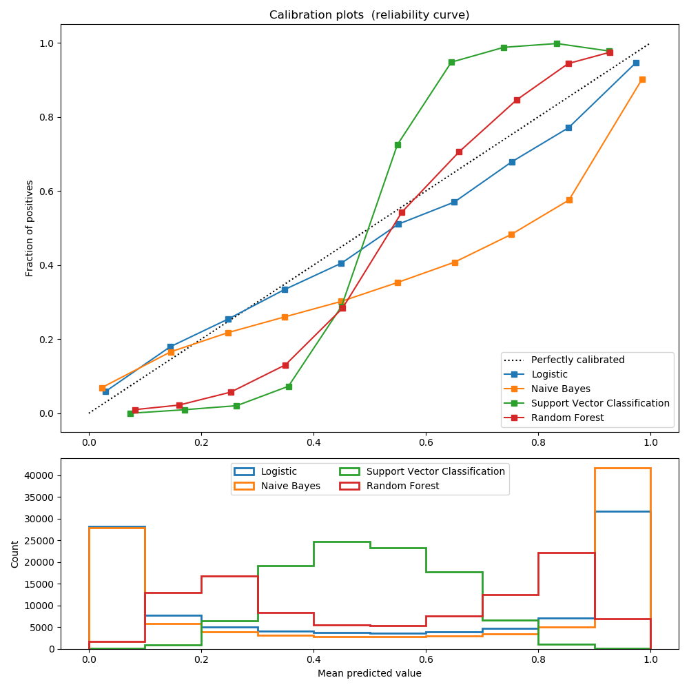
LogisticRegression returns well calibrated predictions by default as it directly
optimizes log-loss. In contrast, the other methods return biased probabilities;
with different biases per method:
GaussianNBtends to push probabilities to 0 or 1 (note the counts in the histograms). This is mainly because it makes the assumption that features are conditionally independent given the class, which is not the case in this dataset which contains 2 redundant features.
RandomForestClassifiershows the opposite behavior: the histograms show peaks at approximately 0.2 and 0.9 probability, while probabilities close to 0 or 1 are very rare. An explanation for this is given by Niculescu-Mizil and Caruana [4]: “Methods such as bagging and random forests that average predictions from a base set of models can have difficulty making predictions near 0 and 1 because variance in the underlying base models will bias predictions that should be near zero or one away from these values. Because predictions are restricted to the interval [0,1], errors caused by variance tend to be one-sided near zero and one. For example, if a model should predict p = 0 for a case, the only way bagging can achieve this is if all bagged trees predict zero. If we add noise to the trees that bagging is averaging over, this noise will cause some trees to predict values larger than 0 for this case, thus moving the average prediction of the bagged ensemble away from 0. We observe this effect most strongly with random forests because the base-level trees trained with random forests have relatively high variance due to feature subsetting.” As a result, the calibration curve also referred to as the reliability diagram (Wilks 1995 [5]) shows a characteristic sigmoid shape, indicating that the classifier could trust its “intuition” more and return probabilities closer to 0 or 1 typically.
- Linear Support Vector Classification (
LinearSVC) shows an even more sigmoid curve as the RandomForestClassifier, which is typical for maximum-margin methods (compare Niculescu-Mizil and Caruana [4]), which focus on hard samples that are close to the decision boundary (the support vectors).
Two approaches for performing calibration of probabilistic predictions are
provided: a parametric approach based on Platt’s sigmoid model and a
non-parametric approach based on isotonic regression (sklearn.isotonic).
Probability calibration should be done on new data not used for model fitting.
The class CalibratedClassifierCV uses a cross-validation generator and
estimates for each split the model parameter on the train samples and the
calibration of the test samples. The probabilities predicted for the
folds are then averaged. Already fitted classifiers can be calibrated by
CalibratedClassifierCV via the parameter cv=”prefit”. In this case,
the user has to take care manually that data for model fitting and calibration
are disjoint.
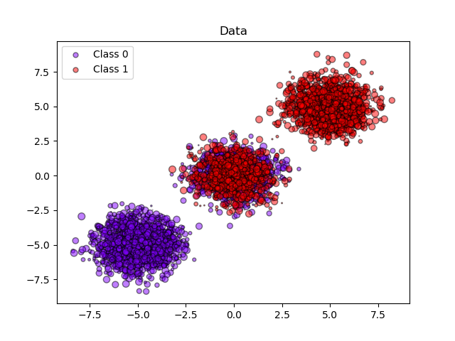
The following images demonstrate the benefit of probability calibration. The first image present a dataset with 2 classes and 3 blobs of data. The blob in the middle contains random samples of each class. The probability for the samples in this blob should be 0.5.
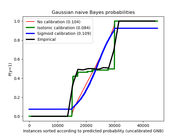
The following image shows on the data above the estimated probability using a Gaussian naive Bayes classifier without calibration, with a sigmoid calibration and with a non-parametric isotonic calibration. One can observe that the non-parametric model provides the most accurate probability estimates for samples in the middle, i.e., 0.5.
The following experiment is performed on an artificial dataset for binary
classification with 100,000 samples (1,000 of them are used for model fitting)
with 20 features. Of the 20 features, only 2 are informative and 10 are
redundant. The figure shows the estimated probabilities obtained with
logistic regression, a linear support-vector classifier (SVC), and linear SVC with
both isotonic calibration and sigmoid calibration.
The Brier score is a metric which is a combination of calibration loss and refinement loss,
brier_score_loss, reported in the legend (the smaller the better).
Calibration loss is defined as the mean squared deviation from empirical probabilities
derived from the slope of ROC segments. Refinement loss can be defined as the expected
optimal loss as measured by the area under the optimal cost curve.
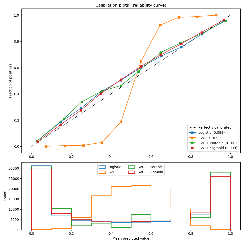
One can observe here that logistic regression is well calibrated as its curve is nearly diagonal. Linear SVC’s calibration curve or reliability diagram has a sigmoid curve, which is typical for an under-confident classifier. In the case of LinearSVC, this is caused by the margin property of the hinge loss, which lets the model focus on hard samples that are close to the decision boundary (the support vectors). Both kinds of calibration can fix this issue and yield nearly identical results. The next figure shows the calibration curve of Gaussian naive Bayes on the same data, with both kinds of calibration and also without calibration.
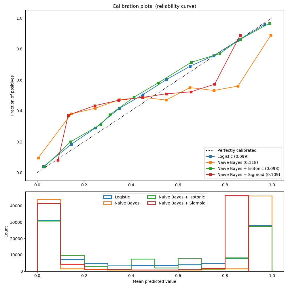
One can see that Gaussian naive Bayes performs very badly but does so in an other way than linear SVC: While linear SVC exhibited a sigmoid calibration curve, Gaussian naive Bayes’ calibration curve has a transposed-sigmoid shape. This is typical for an over-confident classifier. In this case, the classifier’s overconfidence is caused by the redundant features which violate the naive Bayes assumption of feature-independence.
Calibration of the probabilities of Gaussian naive Bayes with isotonic regression can fix this issue as can be seen from the nearly diagonal calibration curve. Sigmoid calibration also improves the brier score slightly, albeit not as strongly as the non-parametric isotonic calibration. This is an intrinsic limitation of sigmoid calibration, whose parametric form assumes a sigmoid rather than a transposed-sigmoid curve. The non-parametric isotonic calibration model, however, makes no such strong assumptions and can deal with either shape, provided that there is sufficient calibration data. In general, sigmoid calibration is preferable in cases where the calibration curve is sigmoid and where there is limited calibration data, while isotonic calibration is preferable for non-sigmoid calibration curves and in situations where large amounts of data are available for calibration.
CalibratedClassifierCV can also deal with classification tasks that
involve more than two classes if the base estimator can do so. In this case,
the classifier is calibrated first for each class separately in an one-vs-rest
fashion. When predicting probabilities for unseen data, the calibrated
probabilities for each class are predicted separately. As those probabilities
do not necessarily sum to one, a postprocessing is performed to normalize them.
The next image illustrates how sigmoid calibration changes predicted probabilities for a 3-class classification problem. Illustrated is the standard 2-simplex, where the three corners correspond to the three classes. Arrows point from the probability vectors predicted by an uncalibrated classifier to the probability vectors predicted by the same classifier after sigmoid calibration on a hold-out validation set. Colors indicate the true class of an instance (red: class 1, green: class 2, blue: class 3).
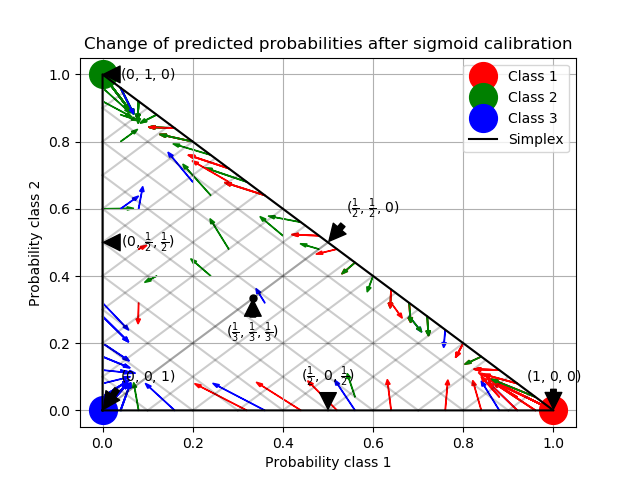
The base classifier is a random forest classifier with 25 base estimators (trees). If this classifier is trained on all 800 training datapoints, it is overly confident in its predictions and thus incurs a large log-loss. Calibrating an identical classifier, which was trained on 600 datapoints, with method=’sigmoid’ on the remaining 200 datapoints reduces the confidence of the predictions, i.e., moves the probability vectors from the edges of the simplex towards the center:
This calibration results in a lower log-loss. Note that an alternative would have been to increase the number of base estimators which would have resulted in a similar decrease in log-loss.
References:
- Obtaining calibrated probability estimates from decision trees and naive Bayesian classifiers, B. Zadrozny & C. Elkan, ICML 2001
- Transforming Classifier Scores into Accurate Multiclass Probability Estimates, B. Zadrozny & C. Elkan, (KDD 2002)
- Probabilistic Outputs for Support Vector Machines and Comparisons to Regularized Likelihood Methods, J. Platt, (1999)
| [4] | (1, 2) Predicting Good Probabilities with Supervised Learning, A. Niculescu-Mizil & R. Caruana, ICML 2005 |
| [5] | On the combination of forecast probabilities for consecutive precipitation periods. Wea. Forecasting, 5, 640–650., Wilks, D. S., 1990a |