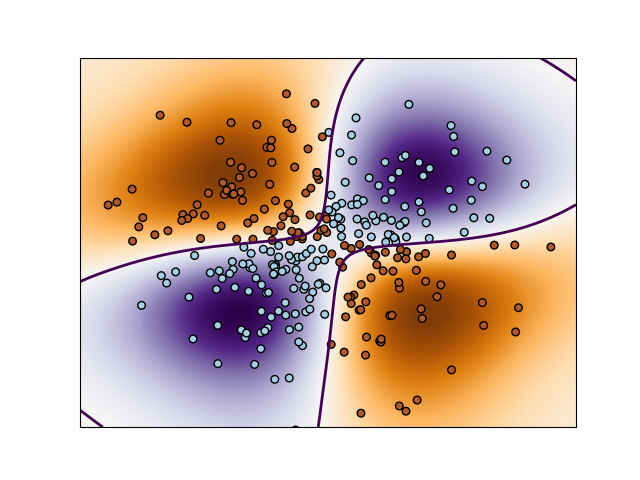
Non-linear SVM

Perform binary classification using non-linear SVC with RBF kernel. The target to predict is a XOR of the inputs.

The color map illustrates the decision function learned by the SVC.

Out:

/home/circleci/project/sklearn/svm/base.py:196: FutureWarning: The default value of gamma will change from 'auto' to 'scale' in version 0.22 to account better for unscaled features. Set gamma explicitly to 'auto' or 'scale' to avoid this warning.
  "avoid this warning.", FutureWarning)
/home/circleci/project/examples/svm/plot_svm_nonlinear.py:36: UserWarning: The following kwargs were not used by contour: 'linetypes'
  linetypes='--')

print(__doc__)

import numpy as np
import matplotlib.pyplot as plt
from sklearn import svm

xx, yy = np.meshgrid(np.linspace(-3, 3, 500),
                     np.linspace(-3, 3, 500))
np.random.seed(0)
X = np.random.randn(300, 2)
Y = np.logical_xor(X[:, 0] > 0, X[:, 1] > 0)

# fit the model
clf = svm.NuSVC()
clf.fit(X, Y)

# plot the decision function for each datapoint on the grid
Z = clf.decision_function(np.c_[xx.ravel(), yy.ravel()])
Z = Z.reshape(xx.shape)

plt.imshow(Z, interpolation='nearest',
           extent=(xx.min(), xx.max(), yy.min(), yy.max()), aspect='auto',
           origin='lower', cmap=plt.cm.PuOr_r)
contours = plt.contour(xx, yy, Z, levels=[0], linewidths=2,
                       linetypes='--')
plt.scatter(X[:, 0], X[:, 1], s=30, c=Y, cmap=plt.cm.Paired,
            edgecolors='k')
plt.xticks(())
plt.yticks(())
plt.axis([-3, 3, -3, 3])
plt.show()