
Note
Click here to download the full example code
Visualization of MLP weights on MNIST
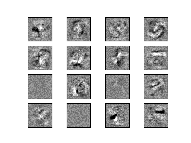
Sometimes looking at the learned coefficients of a neural network can provide insight into the learning behavior. For example if weights look unstructured, maybe some were not used at all, or if very large coefficients exist, maybe regularization was too low or the learning rate too high.
This example shows how to plot some of the first layer weights in a MLPClassifier trained on the MNIST dataset.
The input data consists of 28x28 pixel handwritten digits, leading to 784 features in the dataset. Therefore the first layer weight matrix have the shape (784, hidden_layer_sizes[0]). We can therefore visualize a single column of the weight matrix as a 28x28 pixel image.
To make the example run faster, we use very few hidden units, and train only for a very short time. Training longer would result in weights with a much smoother spatial appearance.
Out:
Iteration 1, loss = 0.32009978
Iteration 2, loss = 0.15347534
Iteration 3, loss = 0.11544755
Iteration 4, loss = 0.09279764
Iteration 5, loss = 0.07889367
Iteration 6, loss = 0.07170497
Iteration 7, loss = 0.06282111
Iteration 8, loss = 0.05529723
Iteration 9, loss = 0.04960484
Iteration 10, loss = 0.04645355
/home/circleci/project/sklearn/neural_network/multilayer_perceptron.py:562: ConvergenceWarning: Stochastic Optimizer: Maximum iterations (10) reached and the optimization hasn't converged yet.
  % self.max_iter, ConvergenceWarning)
Training set score: 0.986800
Test set score: 0.970000
import matplotlib.pyplot as plt
from sklearn.datasets import fetch_openml
from sklearn.neural_network import MLPClassifier

print(__doc__)

# Load data from https://www.openml.org/d/554
X, y = fetch_openml('mnist_784', version=1, return_X_y=True)
X = X / 255.

# rescale the data, use the traditional train/test split
X_train, X_test = X[:60000], X[60000:]
y_train, y_test = y[:60000], y[60000:]

# mlp = MLPClassifier(hidden_layer_sizes=(100, 100), max_iter=400, alpha=1e-4,
#                     solver='sgd', verbose=10, tol=1e-4, random_state=1)
mlp = MLPClassifier(hidden_layer_sizes=(50,), max_iter=10, alpha=1e-4,
                    solver='sgd', verbose=10, tol=1e-4, random_state=1,
                    learning_rate_init=.1)

mlp.fit(X_train, y_train)
print("Training set score: %f" % mlp.score(X_train, y_train))
print("Test set score: %f" % mlp.score(X_test, y_test))

fig, axes = plt.subplots(4, 4)
# use global min / max to ensure all weights are shown on the same scale
vmin, vmax = mlp.coefs_[0].min(), mlp.coefs_[0].max()
for coef, ax in zip(mlp.coefs_[0].T, axes.ravel()):
    ax.matshow(coef.reshape(28, 28), cmap=plt.cm.gray, vmin=.5 * vmin,
               vmax=.5 * vmax)
    ax.set_xticks(())
    ax.set_yticks(())

plt.show()
Total running time of the script: ( 0 minutes 43.042 seconds)