Bayesian Ridge Regression

Computes a Bayesian Ridge Regression on a synthetic dataset.

See Bayesian Ridge Regression for more information on the regressor.

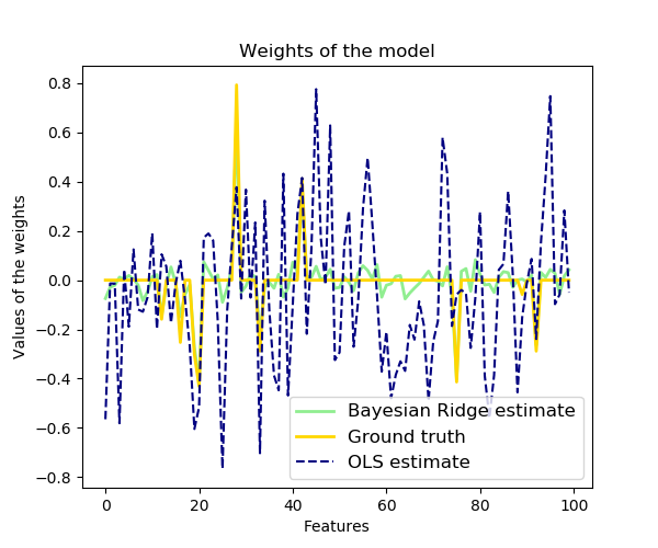
Compared to the OLS (ordinary least squares) estimator, the coefficient weights are slightly shifted toward zeros, which stabilises them.

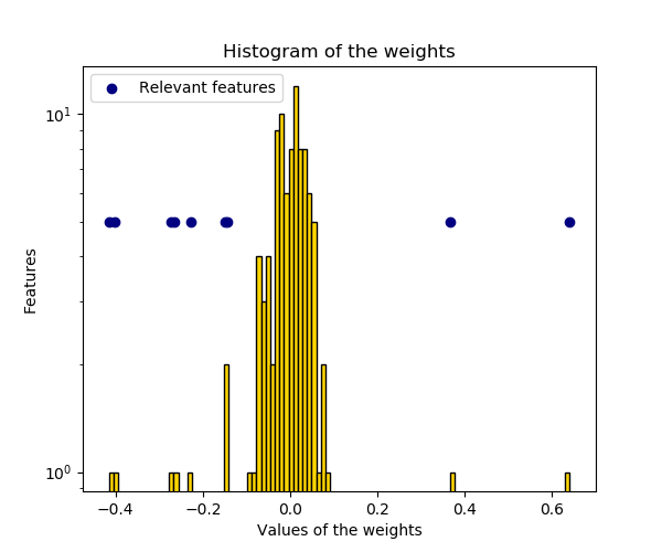
As the prior on the weights is a Gaussian prior, the histogram of the estimated weights is Gaussian.

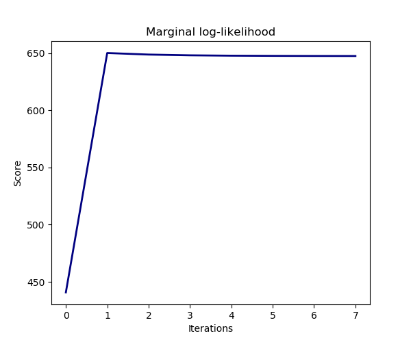
The estimation of the model is done by iteratively maximizing the marginal log-likelihood of the observations.

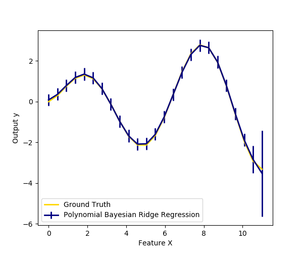
We also plot predictions and uncertainties for Bayesian Ridge Regression for one dimensional regression using polynomial feature expansion. Note the uncertainty starts going up on the right side of the plot. This is because these test samples are outside of the range of the training samples.

• 
• 
• 
• 

Out:

print(__doc__)

import numpy as np
import matplotlib.pyplot as plt
from scipy import stats

from sklearn.linear_model import BayesianRidge, LinearRegression

# #############################################################################
# Generating simulated data with Gaussian weights
np.random.seed(0)
n_samples, n_features = 100, 100
X = np.random.randn(n_samples, n_features)  # Create Gaussian data
# Create weights with a precision lambda_ of 4.
lambda_ = 4.
w = np.zeros(n_features)
# Only keep 10 weights of interest
relevant_features = np.random.randint(0, n_features, 10)
for i in relevant_features:
    w[i] = stats.norm.rvs(loc=0, scale=1. / np.sqrt(lambda_))
# Create noise with a precision alpha of 50.
alpha_ = 50.
noise = stats.norm.rvs(loc=0, scale=1. / np.sqrt(alpha_), size=n_samples)
# Create the target
y = np.dot(X, w) + noise

# #############################################################################
# Fit the Bayesian Ridge Regression and an OLS for comparison
clf = BayesianRidge(compute_score=True)
clf.fit(X, y)

ols = LinearRegression()
ols.fit(X, y)

# #############################################################################
# Plot true weights, estimated weights, histogram of the weights, and
# predictions with standard deviations
lw = 2
plt.figure(figsize=(6, 5))
plt.title("Weights of the model")
plt.plot(clf.coef_, color='lightgreen', linewidth=lw,
         label="Bayesian Ridge estimate")
plt.plot(w, color='gold', linewidth=lw, label="Ground truth")
plt.plot(ols.coef_, color='navy', linestyle='--', label="OLS estimate")
plt.xlabel("Features")
plt.ylabel("Values of the weights")
plt.legend(loc="best", prop=dict(size=12))

plt.figure(figsize=(6, 5))
plt.title("Histogram of the weights")
plt.hist(clf.coef_, bins=n_features, color='gold', log=True,
         edgecolor='black')
plt.scatter(clf.coef_[relevant_features], np.full(len(relevant_features), 5.),
            color='navy', label="Relevant features")
plt.ylabel("Features")
plt.xlabel("Values of the weights")
plt.legend(loc="upper left")

plt.figure(figsize=(6, 5))
plt.title("Marginal log-likelihood")
plt.plot(clf.scores_, color='navy', linewidth=lw)
plt.ylabel("Score")
plt.xlabel("Iterations")


# Plotting some predictions for polynomial regression
def f(x, noise_amount):
    y = np.sqrt(x) * np.sin(x)
    noise = np.random.normal(0, 1, len(x))
    return y + noise_amount * noise


degree = 10
X = np.linspace(0, 10, 100)
y = f(X, noise_amount=0.1)
clf_poly = BayesianRidge()
clf_poly.fit(np.vander(X, degree), y)

X_plot = np.linspace(0, 11, 25)
y_plot = f(X_plot, noise_amount=0)
y_mean, y_std = clf_poly.predict(np.vander(X_plot, degree), return_std=True)
plt.figure(figsize=(6, 5))
plt.errorbar(X_plot, y_mean, y_std, color='navy',
             label="Polynomial Bayesian Ridge Regression", linewidth=lw)
plt.plot(X_plot, y_plot, color='gold', linewidth=lw,
         label="Ground Truth")
plt.ylabel("Output y")
plt.xlabel("Feature X")
plt.legend(loc="lower left")
plt.show()