This is documentation for an old release of Scikit-learn (version 0.20). Try the latest stable release (version 1.6) or development (unstable) versions.

The Iris Dataset

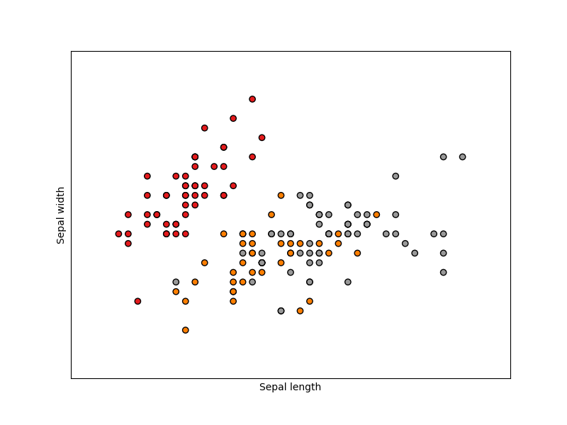
This data sets consists of 3 different types of irises’ (Setosa, Versicolour, and Virginica) petal and sepal length, stored in a 150x4 numpy.ndarray

The rows being the samples and the columns being: Sepal Length, Sepal Width, Petal Length and Petal Width.

The below plot uses the first two features. See here for more information on this dataset.

• 
• 

Out:

print(__doc__)


# Code source: Gaël Varoquaux
# Modified for documentation by Jaques Grobler
# License: BSD 3 clause

import matplotlib.pyplot as plt
from mpl_toolkits.mplot3d import Axes3D
from sklearn import datasets
from sklearn.decomposition import PCA

# import some data to play with
iris = datasets.load_iris()
X = iris.data[:, :2]  # we only take the first two features.
y = iris.target

x_min, x_max = X[:, 0].min() - .5, X[:, 0].max() + .5
y_min, y_max = X[:, 1].min() - .5, X[:, 1].max() + .5

plt.figure(2, figsize=(8, 6))
plt.clf()

# Plot the training points
plt.scatter(X[:, 0], X[:, 1], c=y, cmap=plt.cm.Set1,
            edgecolor='k')
plt.xlabel('Sepal length')
plt.ylabel('Sepal width')

plt.xlim(x_min, x_max)
plt.ylim(y_min, y_max)
plt.xticks(())
plt.yticks(())

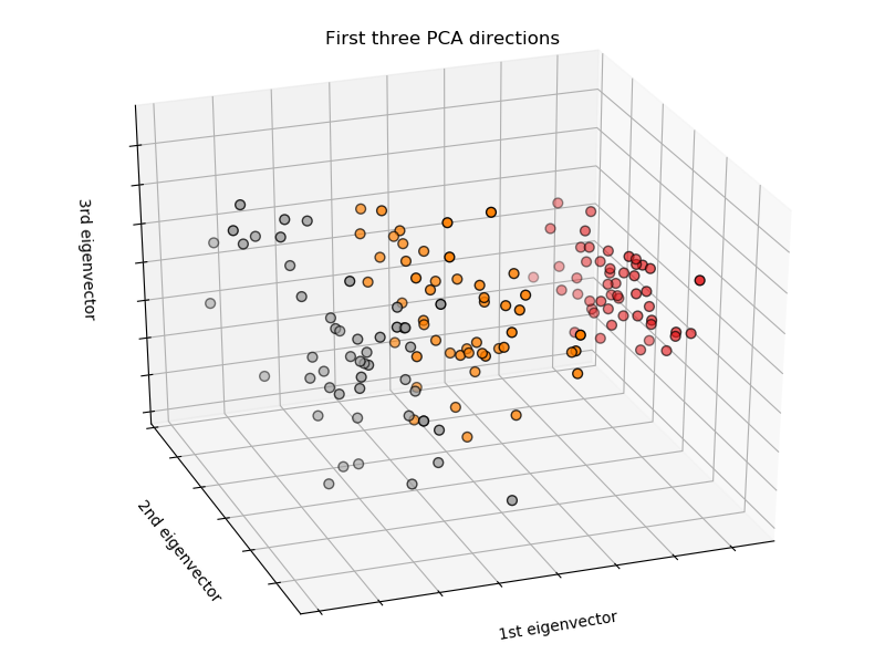
# To getter a better understanding of interaction of the dimensions
# plot the first three PCA dimensions
fig = plt.figure(1, figsize=(8, 6))
ax = Axes3D(fig, elev=-150, azim=110)
X_reduced = PCA(n_components=3).fit_transform(iris.data)
ax.scatter(X_reduced[:, 0], X_reduced[:, 1], X_reduced[:, 2], c=y,
           cmap=plt.cm.Set1, edgecolor='k', s=40)
ax.set_title("First three PCA directions")
ax.set_xlabel("1st eigenvector")
ax.w_xaxis.set_ticklabels([])
ax.set_ylabel("2nd eigenvector")
ax.w_yaxis.set_ticklabels([])
ax.set_zlabel("3rd eigenvector")
ax.w_zaxis.set_ticklabels([])

plt.show()