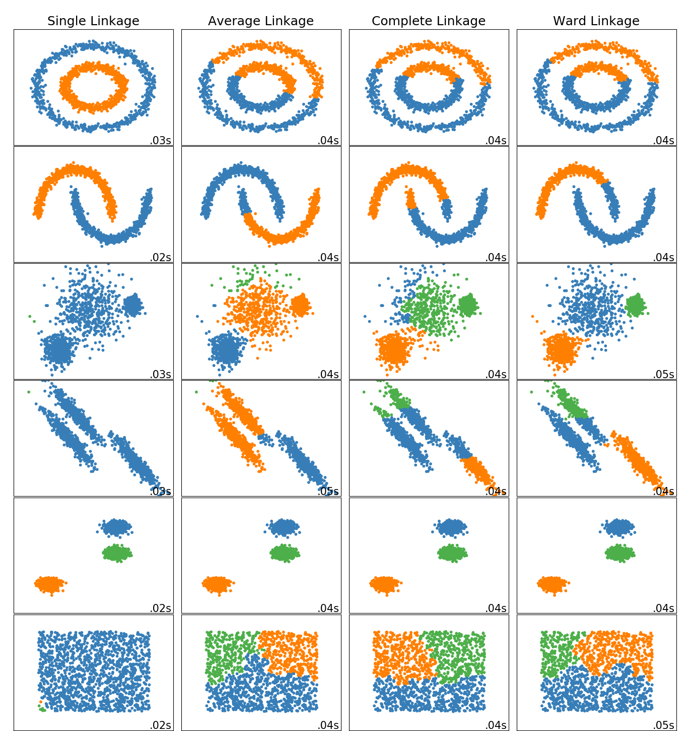
Comparing different hierarchical linkage methods on toy datasets

This example shows characteristics of different linkage methods for hierarchical clustering on datasets that are “interesting” but still in 2D.

The main observations to make are:

• single linkage is fast, and can perform well on non-globular data, but it performs poorly in the presence of noise.
• average and complete linkage perform well on cleanly separated globular clusters, but have mixed results otherwise.
• Ward is the most effective method for noisy data.

While these examples give some intuition about the algorithms, this intuition might not apply to very high dimensional data.

print(__doc__)

import time
import warnings

import numpy as np
import matplotlib.pyplot as plt

from sklearn import cluster, datasets
from sklearn.preprocessing import StandardScaler
from itertools import cycle, islice

np.random.seed(0)

Out:

Generate datasets. We choose the size big enough to see the scalability of the algorithms, but not too big to avoid too long running times

n_samples = 1500
noisy_circles = datasets.make_circles(n_samples=n_samples, factor=.5,
                                      noise=.05)
noisy_moons = datasets.make_moons(n_samples=n_samples, noise=.05)
blobs = datasets.make_blobs(n_samples=n_samples, random_state=8)
no_structure = np.random.rand(n_samples, 2), None

# Anisotropicly distributed data
random_state = 170
X, y = datasets.make_blobs(n_samples=n_samples, random_state=random_state)
transformation = [[0.6, -0.6], [-0.4, 0.8]]
X_aniso = np.dot(X, transformation)
aniso = (X_aniso, y)

# blobs with varied variances
varied = datasets.make_blobs(n_samples=n_samples,
                             cluster_std=[1.0, 2.5, 0.5],
                             random_state=random_state)

Run the clustering and plot

# Set up cluster parameters
plt.figure(figsize=(9 * 1.3 + 2, 14.5))
plt.subplots_adjust(left=.02, right=.98, bottom=.001, top=.96, wspace=.05,
                    hspace=.01)

plot_num = 1

default_base = {'n_neighbors': 10,
                'n_clusters': 3}

datasets = [
    (noisy_circles, {'n_clusters': 2}),
    (noisy_moons, {'n_clusters': 2}),
    (varied, {'n_neighbors': 2}),
    (aniso, {'n_neighbors': 2}),
    (blobs, {}),
    (no_structure, {})]

for i_dataset, (dataset, algo_params) in enumerate(datasets):
    # update parameters with dataset-specific values
    params = default_base.copy()
    params.update(algo_params)

    X, y = dataset

    # normalize dataset for easier parameter selection
    X = StandardScaler().fit_transform(X)

    # ============
    # Create cluster objects
    # ============
    ward = cluster.AgglomerativeClustering(
        n_clusters=params['n_clusters'], linkage='ward')
    complete = cluster.AgglomerativeClustering(
        n_clusters=params['n_clusters'], linkage='complete')
    average = cluster.AgglomerativeClustering(
        n_clusters=params['n_clusters'], linkage='average')
    single = cluster.AgglomerativeClustering(
        n_clusters=params['n_clusters'], linkage='single')

    clustering_algorithms = (
        ('Single Linkage', single),
        ('Average Linkage', average),
        ('Complete Linkage', complete),
        ('Ward Linkage', ward),
    )

    for name, algorithm in clustering_algorithms:
        t0 = time.time()

        # catch warnings related to kneighbors_graph
        with warnings.catch_warnings():
            warnings.filterwarnings(
                "ignore",
                message="the number of connected components of the " +
                "connectivity matrix is [0-9]{1,2}" +
                " > 1. Completing it to avoid stopping the tree early.",
                category=UserWarning)
            algorithm.fit(X)

        t1 = time.time()
        if hasattr(algorithm, 'labels_'):
            y_pred = algorithm.labels_.astype(np.int)
        else:
            y_pred = algorithm.predict(X)

        plt.subplot(len(datasets), len(clustering_algorithms), plot_num)
        if i_dataset == 0:
            plt.title(name, size=18)

        colors = np.array(list(islice(cycle(['#377eb8', '#ff7f00', '#4daf4a',
                                             '#f781bf', '#a65628', '#984ea3',
                                             '#999999', '#e41a1c', '#dede00']),
                                      int(max(y_pred) + 1))))
        plt.scatter(X[:, 0], X[:, 1], s=10, color=colors[y_pred])

        plt.xlim(-2.5, 2.5)
        plt.ylim(-2.5, 2.5)
        plt.xticks(())
        plt.yticks(())
        plt.text(.99, .01, ('%.2fs' % (t1 - t0)).lstrip('0'),
                 transform=plt.gca().transAxes, size=15,
                 horizontalalignment='right')
        plot_num += 1

plt.show()