1.2. Linear and Quadratic Discriminant Analysis¶

Linear Discriminant Analysis (discriminant_analysis.LinearDiscriminantAnalysis) and Quadratic Discriminant Analysis (discriminant_analysis.QuadraticDiscriminantAnalysis) are two classic classifiers, with, as their names suggest, a linear and a quadratic decision surface, respectively.

These classifiers are attractive because they have closed-form solutions that can be easily computed, are inherently multiclass, have proven to work well in practice and have no hyperparameters to tune.

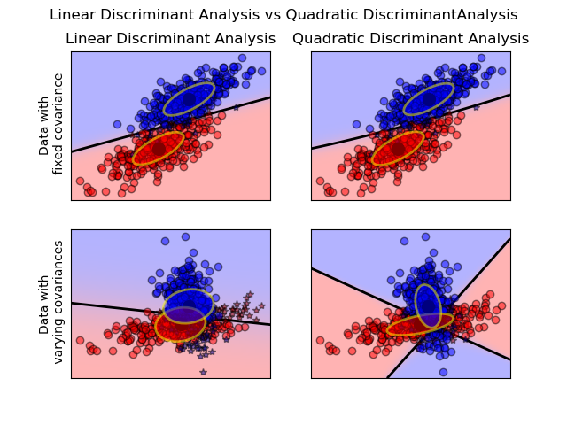
The plot shows decision boundaries for Linear Discriminant Analysis and Quadratic Discriminant Analysis. The bottom row demonstrates that Linear Discriminant Analysis can only learn linear boundaries, while Quadratic Discriminant Analysis can learn quadratic boundaries and is therefore more flexible.

Examples:

Linear and Quadratic Discriminant Analysis with covariance ellipsoid: Comparison of LDA and QDA on synthetic data.

1.2.1. Dimensionality reduction using Linear Discriminant Analysis¶

discriminant_analysis.LinearDiscriminantAnalysis can be used to perform supervised dimensionality reduction, by projecting the input data to a linear subspace consisting of the directions which maximize the separation between classes (in a precise sense discussed in the mathematics section below). The dimension of the output is necessarily less than the number of classes, so this is a in general a rather strong dimensionality reduction, and only makes senses in a multiclass setting.

This is implemented in discriminant_analysis.LinearDiscriminantAnalysis.transform. The desired dimensionality can be set using the n_components constructor parameter. This parameter has no influence on discriminant_analysis.LinearDiscriminantAnalysis.fit or discriminant_analysis.LinearDiscriminantAnalysis.predict.

Examples:

Comparison of LDA and PCA 2D projection of Iris dataset: Comparison of LDA and PCA for dimensionality reduction of the Iris dataset

1.2.2. Mathematical formulation of the LDA and QDA classifiers¶

Both LDA and QDA can be derived from simple probabilistic models which model the class conditional distribution of the data $P(X|y=k)$ for each class $k$ . Predictions can then be obtained by using Bayes’ rule:

$P(y=k | X) = \frac{P(X | y=k) P(y=k)}{P(X)} = \frac{P(X | y=k) P(y = k)}{ \sum_{l} P(X | y=l) \cdot P(y=l)}$

and we select the class $k$ which maximizes this conditional probability.

More specifically, for linear and quadratic discriminant analysis, $P(X|y)$ is modelled as a multivariate Gaussian distribution with density:

$p(X | y=k) = \frac{1}{(2\pi)^n |\Sigma_k|^{1/2}}\exp\left(-\frac{1}{2} (X-\mu_k)^t \Sigma_k^{-1} (X-\mu_k)\right)$

To use this model as a classifier, we just need to estimate from the training data the class priors $P(y=k)$ (by the proportion of instances of class $k$ ), the class means $\mu_k$ (by the empirical sample class means) and the covariance matrices (either by the empirical sample class covariance matrices, or by a regularized estimator: see the section on shrinkage below).

In the case of LDA, the Gaussians for each class are assumed to share the same covariance matrix: $\Sigma_k = \Sigma$ for all $k$ . This leads to linear decision surfaces between, as can be seen by comparing the log-probability ratios $\log[P(y=k | X) / P(y=l | X)]$ :

$\log\left(\frac{P(y=k|X)}{P(y=l | X)}\right) = 0 \Leftrightarrow (\mu_k-\mu_l)\Sigma^{-1} X = \frac{1}{2} (\mu_k^t \Sigma^{-1} \mu_k - \mu_l^t \Sigma^{-1} \mu_l)$

In the case of QDA, there are no assumptions on the covariance matrices $\Sigma_k$ of the Gaussians, leading to quadratic decision surfaces. See [3] for more details.

Note

Relation with Gaussian Naive Bayes

If in the QDA model one assumes that the covariance matrices are diagonal, then the inputs are assumed to be conditionally independent in each class, and the resulting classifier is equivalent to the Gaussian Naive Bayes classifier naive_bayes.GaussianNB.

1.2.3. Mathematical formulation of LDA dimensionality reduction¶

To understand the use of LDA in dimensionality reduction, it is useful to start with a geometric reformulation of the LDA classification rule explained above. We write $K$ for the total number of target classes. Since in LDA we assume that all classes have the same estimated covariance $\Sigma$ , we can rescale the data so that this covariance is the identity:

$X^* = D^{-1/2}U^t X\text{ with }\Sigma = UDU^t$

Then one can show that to classify a data point after scaling is equivalent to finding the estimated class mean $\mu^*_k$ which is closest to the data point in the Euclidean distance. But this can be done just as well after projecting on the $K-1$ affine subspace $H_K$ generated by all the $\mu^*_k$ for all classes. This shows that, implicit in the LDA classifier, there is a dimensionality reduction by linear projection onto a $K-1$ dimensional space.

We can reduce the dimension even more, to a chosen $L$ , by projecting onto the linear subspace $H_L$ which maximize the variance of the $\mu^*_k$ after projection (in effect, we are doing a form of PCA for the transformed class means $\mu^*_k$ ). This $L$ corresponds to the n_components parameter used in the discriminant_analysis.LinearDiscriminantAnalysis.transform method. See [3] for more details.

1.2.4. Shrinkage¶

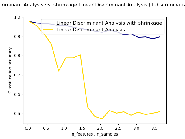
Shrinkage is a tool to improve estimation of covariance matrices in situations where the number of training samples is small compared to the number of features. In this scenario, the empirical sample covariance is a poor estimator. Shrinkage LDA can be used by setting the shrinkage parameter of the discriminant_analysis.LinearDiscriminantAnalysis class to ‘auto’. This automatically determines the optimal shrinkage parameter in an analytic way following the lemma introduced by Ledoit and Wolf [4]. Note that currently shrinkage only works when setting the solver parameter to ‘lsqr’ or ‘eigen’.

The shrinkage parameter can also be manually set between 0 and 1. In particular, a value of 0 corresponds to no shrinkage (which means the empirical covariance matrix will be used) and a value of 1 corresponds to complete shrinkage (which means that the diagonal matrix of variances will be used as an estimate for the covariance matrix). Setting this parameter to a value between these two extrema will estimate a shrunk version of the covariance matrix.

1.2.5. Estimation algorithms¶

The default solver is ‘svd’. It can perform both classification and transform, and it does not rely on the calculation of the covariance matrix. This can be an advantage in situations where the number of features is large. However, the ‘svd’ solver cannot be used with shrinkage.

The ‘lsqr’ solver is an efficient algorithm that only works for classification. It supports shrinkage.

The ‘eigen’ solver is based on the optimization of the between class scatter to within class scatter ratio. It can be used for both classification and transform, and it supports shrinkage. However, the ‘eigen’ solver needs to compute the covariance matrix, so it might not be suitable for situations with a high number of features.

Examples:

Normal and Shrinkage Linear Discriminant Analysis for classification: Comparison of LDA classifiers with and without shrinkage.

References:

[3]	(1, 2) “The Elements of Statistical Learning”, Hastie T., Tibshirani R., Friedman J., Section 4.3, p.106-119, 2008.

[4]	Ledoit O, Wolf M. Honey, I Shrunk the Sample Covariance Matrix. The Journal of Portfolio Management 30(4), 110-119, 2004.