sklearn.mixture.BayesianGaussianMixture

class sklearn.mixture.BayesianGaussianMixture(n_components=1, covariance_type=’full’, tol=0.001, reg_covar=1e-06, max_iter=100, n_init=1, init_params=’kmeans’, weight_concentration_prior_type=’dirichlet_process’, weight_concentration_prior=None, mean_precision_prior=None, mean_prior=None, degrees_of_freedom_prior=None, covariance_prior=None, random_state=None, warm_start=False, verbose=0, verbose_interval=10)

Variational Bayesian estimation of a Gaussian mixture.

This class allows to infer an approximate posterior distribution over the parameters of a Gaussian mixture distribution. The effective number of components can be inferred from the data.

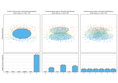
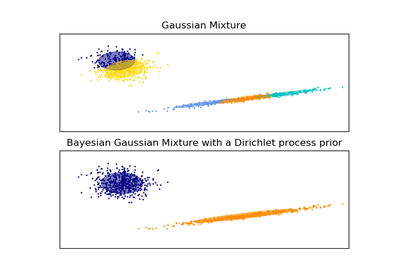
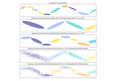
This class implements two types of prior for the weights distribution: a finite mixture model with Dirichlet distribution and an infinite mixture model with the Dirichlet Process. In practice Dirichlet Process inference algorithm is approximated and uses a truncated distribution with a fixed maximum number of components (called the Stick-breaking representation). The number of components actually used almost always depends on the data.

New in version 0.18.

Read more in the User Guide.

Parameters:

n_components : int, defaults to 1.

The number of mixture components. Depending on the data and the value of the weight_concentration_prior the model can decide to not use all the components by setting some component weights_ to values very close to zero. The number of effective components is therefore smaller than n_components.

covariance_type : {‘full’, ‘tied’, ‘diag’, ‘spherical’}, defaults to ‘full’

String describing the type of covariance parameters to use. Must be one of:

'full' (each component has its own general covariance matrix),
'tied' (all components share the same general covariance matrix),
'diag' (each component has its own diagonal covariance matrix),
'spherical' (each component has its own single variance).

tol : float, defaults to 1e-3.

The convergence threshold. EM iterations will stop when the lower bound average gain on the likelihood (of the training data with respect to the model) is below this threshold.

reg_covar : float, defaults to 1e-6.

Non-negative regularization added to the diagonal of covariance. Allows to assure that the covariance matrices are all positive.

max_iter : int, defaults to 100.

The number of EM iterations to perform.

n_init : int, defaults to 1.

The number of initializations to perform. The result with the highest lower bound value on the likelihood is kept.

init_params : {‘kmeans’, ‘random’}, defaults to ‘kmeans’.

The method used to initialize the weights, the means and the covariances. Must be one of:

'kmeans' : responsibilities are initialized using kmeans.
'random' : responsibilities are initialized randomly.

weight_concentration_prior_type : str, defaults to ‘dirichlet_process’.

String describing the type of the weight concentration prior. Must be one of:

'dirichlet_process' (using the Stick-breaking representation),
'dirichlet_distribution' (can favor more uniform weights).

weight_concentration_prior : float | None, optional.

The dirichlet concentration of each component on the weight distribution (Dirichlet). This is commonly called gamma in the literature. The higher concentration puts more mass in the center and will lead to more components being active, while a lower concentration parameter will lead to more mass at the edge of the mixture weights simplex. The value of the parameter must be greater than 0. If it is None, it’s set to 1. / n_components.

mean_precision_prior : float | None, optional.

The precision prior on the mean distribution (Gaussian). Controls the extend to where means can be placed. Smaller values concentrate the means of each clusters around mean_prior. The value of the parameter must be greater than 0. If it is None, it’s set to 1.

mean_prior : array-like, shape (n_features,), optional

The prior on the mean distribution (Gaussian). If it is None, it’s set to the mean of X.

degrees_of_freedom_prior : float | None, optional.

The prior of the number of degrees of freedom on the covariance distributions (Wishart). If it is None, it’s set to n_features.

covariance_prior : float or array-like, optional

The prior on the covariance distribution (Wishart). If it is None, the emiprical covariance prior is initialized using the covariance of X. The shape depends on covariance_type:

(n_features, n_features) if 'full',
(n_features, n_features) if 'tied',
(n_features)             if 'diag',
float                    if 'spherical'

random_state : int, RandomState instance or None, optional (default=None)

If int, random_state is the seed used by the random number generator; If RandomState instance, random_state is the random number generator; If None, the random number generator is the RandomState instance used by np.random.

warm_start : bool, default to False.

If ‘warm_start’ is True, the solution of the last fitting is used as initialization for the next call of fit(). This can speed up convergence when fit is called several time on similar problems.

verbose : int, default to 0.

Enable verbose output. If 1 then it prints the current initialization and each iteration step. If greater than 1 then it prints also the log probability and the time needed for each step.

verbose_interval : int, default to 10.

Number of iteration done before the next print.

Attributes:

weights_ : array-like, shape (n_components,)

The weights of each mixture components.

means_ : array-like, shape (n_components, n_features)

The mean of each mixture component.

covariances_ : array-like

The covariance of each mixture component. The shape depends on covariance_type:

(n_components,)                        if 'spherical',
(n_features, n_features)               if 'tied',
(n_components, n_features)             if 'diag',
(n_components, n_features, n_features) if 'full'

precisions_ : array-like

The precision matrices for each component in the mixture. A precision matrix is the inverse of a covariance matrix. A covariance matrix is symmetric positive definite so the mixture of Gaussian can be equivalently parameterized by the precision matrices. Storing the precision matrices instead of the covariance matrices makes it more efficient to compute the log-likelihood of new samples at test time. The shape depends on covariance_type:

(n_components,)                        if 'spherical',
(n_features, n_features)               if 'tied',
(n_components, n_features)             if 'diag',
(n_components, n_features, n_features) if 'full'

precisions_cholesky_ : array-like

The cholesky decomposition of the precision matrices of each mixture component. A precision matrix is the inverse of a covariance matrix. A covariance matrix is symmetric positive definite so the mixture of Gaussian can be equivalently parameterized by the precision matrices. Storing the precision matrices instead of the covariance matrices makes it more efficient to compute the log-likelihood of new samples at test time. The shape depends on covariance_type:

(n_components,)                        if 'spherical',
(n_features, n_features)               if 'tied',
(n_components, n_features)             if 'diag',
(n_components, n_features, n_features) if 'full'

converged_ : bool

True when convergence was reached in fit(), False otherwise.

n_iter_ : int

Number of step used by the best fit of inference to reach the convergence.

lower_bound_ : float

Lower bound value on the likelihood (of the training data with respect to the model) of the best fit of inference.

weight_concentration_prior_ : tuple or float

The dirichlet concentration of each component on the weight distribution (Dirichlet). The type depends on weight_concentration_prior_type:

(float, float) if 'dirichlet_process' (Beta parameters),
float          if 'dirichlet_distribution' (Dirichlet parameters).

The higher concentration puts more mass in the center and will lead to more components being active, while a lower concentration parameter will lead to more mass at the edge of the simplex.

weight_concentration_ : array-like, shape (n_components,)

The dirichlet concentration of each component on the weight distribution (Dirichlet).

mean_precision_prior : float

The precision prior on the mean distribution (Gaussian). Controls the extend to where means can be placed. Smaller values concentrate the means of each clusters around mean_prior.

mean_precision_ : array-like, shape (n_components,)

The precision of each components on the mean distribution (Gaussian).

means_prior_ : array-like, shape (n_features,)

The prior on the mean distribution (Gaussian).

degrees_of_freedom_prior_ : float

The prior of the number of degrees of freedom on the covariance distributions (Wishart).

degrees_of_freedom_ : array-like, shape (n_components,)

The number of degrees of freedom of each components in the model.

covariance_prior_ : float or array-like

The prior on the covariance distribution (Wishart). The shape depends on covariance_type:

(n_features, n_features) if 'full',
(n_features, n_features) if 'tied',
(n_features)             if 'diag',
float                    if 'spherical'

See also

GaussianMixture

Finite Gaussian mixture fit with EM.

References

[R236]

Bishop, Christopher M. (2006). “Pattern recognition and machine learning”. Vol. 4 No. 4. New York: Springer.

[R237]

Hagai Attias. (2000). “A Variational Bayesian Framework for Graphical Models”. In Advances in Neural Information Processing Systems 12.

[R238]

Blei, David M. and Michael I. Jordan. (2006). “Variational inference for Dirichlet process mixtures”. Bayesian analysis 1.1

Methods

fit(X[, y])	Estimate model parameters with the EM algorithm.
get_params([deep])	Get parameters for this estimator.
predict(X)	Predict the labels for the data samples in X using trained model.
predict_proba(X)	Predict posterior probability of each component given the data.
sample([n_samples])	Generate random samples from the fitted Gaussian distribution.
score(X[, y])	Compute the per-sample average log-likelihood of the given data X.
score_samples(X)	Compute the weighted log probabilities for each sample.
set_params(**params)	Set the parameters of this estimator.

__init__(n_components=1, covariance_type=’full’, tol=0.001, reg_covar=1e-06, max_iter=100, n_init=1, init_params=’kmeans’, weight_concentration_prior_type=’dirichlet_process’, weight_concentration_prior=None, mean_precision_prior=None, mean_prior=None, degrees_of_freedom_prior=None, covariance_prior=None, random_state=None, warm_start=False, verbose=0, verbose_interval=10)

fit(X, y=None)

Estimate model parameters with the EM algorithm.

The method fit the model n_init times and set the parameters with which the model has the largest likelihood or lower bound. Within each trial, the method iterates between E-step and M-step for max_iter times until the change of likelihood or lower bound is less than tol, otherwise, a ConvergenceWarning is raised.

Parameters:

X : array-like, shape (n_samples, n_features)

List of n_features-dimensional data points. Each row corresponds to a single data point.

Returns:

self :

get_params(deep=True)

Get parameters for this estimator.

Parameters:

deep : boolean, optional

If True, will return the parameters for this estimator and contained subobjects that are estimators.

Returns:

params : mapping of string to any

Parameter names mapped to their values.

predict(X)

Predict the labels for the data samples in X using trained model.

Parameters:

X : array-like, shape (n_samples, n_features)

List of n_features-dimensional data points. Each row corresponds to a single data point.

Returns:

labels : array, shape (n_samples,)

Component labels.

predict_proba(X)

Predict posterior probability of each component given the data.

Parameters:

X : array-like, shape (n_samples, n_features)

List of n_features-dimensional data points. Each row corresponds to a single data point.

Returns:

resp : array, shape (n_samples, n_components)

Returns the probability each Gaussian (state) in the model given each sample.

sample(n_samples=1)

Generate random samples from the fitted Gaussian distribution.

Parameters:

n_samples : int, optional

Number of samples to generate. Defaults to 1.

Returns:

X : array, shape (n_samples, n_features)

Randomly generated sample

y : array, shape (nsamples,)

Component labels

score(X, y=None)

Compute the per-sample average log-likelihood of the given data X.

Parameters:

X : array-like, shape (n_samples, n_dimensions)

List of n_features-dimensional data points. Each row corresponds to a single data point.

Returns:

log_likelihood : float

Log likelihood of the Gaussian mixture given X.

score_samples(X)

Compute the weighted log probabilities for each sample.

Parameters:

X : array-like, shape (n_samples, n_features)

List of n_features-dimensional data points. Each row corresponds to a single data point.

Returns:

log_prob : array, shape (n_samples,)

Log probabilities of each data point in X.

set_params(**params)

Set the parameters of this estimator.

The method works on simple estimators as well as on nested objects (such as pipelines). The latter have parameters of the form <component>__<parameter> so that it’s possible to update each component of a nested object.

Returns:self :

Examples using sklearn.mixture.BayesianGaussianMixture

Concentration Prior Type Analysis of Variation Bayesian Gaussian Mixture

Gaussian Mixture Model Ellipsoids

Gaussian Mixture Model Sine Curve