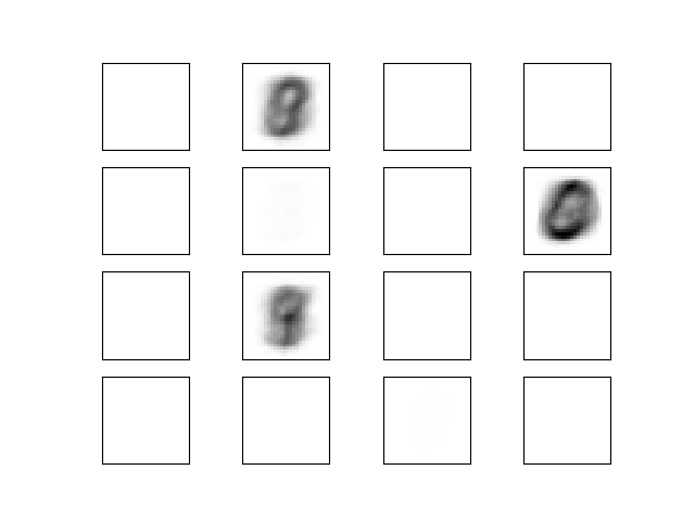
Visualization of MLP weights on MNIST
Sometimes looking at the learned coefficients of a neural network can provide insight into the learning behavior. For example if weights look unstructured, maybe some were not used at all, or if very large coefficients exist, maybe regularization was too low or the learning rate too high.
This example shows how to plot some of the first layer weights in a MLPClassifier trained on the MNIST dataset.
The input data consists of 28x28 pixel handwritten digits, leading to 784 features in the dataset. Therefore the first layer weight matrix have the shape (784, hidden_layer_sizes[0]). We can therefore visualize a single column of the weight matrix as a 28x28 pixel image.
To make the example run faster, we use very few hidden units, and train only for a very short time. Training longer would result in weights with a much smoother spatial appearance.

Out:
________________________________________________________________________________
[Memory] Calling __main__--home-ubuntu-scikit-learn-examples-neural_networks-<string>.fetch_mnist...
fetch_mnist()
_____________________________________________________fetch_mnist - 41.1s, 0.7min
Iteration 1, loss = 88770.19492622
Iteration 2, loss = 94144.72785948
Iteration 3, loss = 94116.48942606
Iteration 4, loss = 94088.25915097
Training loss did not improve more than tol=0.000100 for two consecutive epochs. Stopping.
Training set score: 0.112367
Test set score: 0.113500
import io
from scipy.io.arff import loadarff
import matplotlib.pyplot as plt
from sklearn.datasets import get_data_home
from sklearn.externals.joblib import Memory
from sklearn.neural_network import MLPClassifier
try:
    from urllib.request import urlopen
except ImportError:
    # Python 2
    from urllib2 import urlopen

print(__doc__)

memory = Memory(get_data_home())


@memory.cache()
def fetch_mnist():
    content = urlopen(
        'https://www.openml.org/data/download/52667/mnist_784.arff').read()
    data, meta = loadarff(io.StringIO(content.decode('utf8')))
    data = data.view([('pixels', '<f8', 784), ('class', '|S1')])
    return data['pixels'], data['class']

X, y = fetch_mnist()
# rescale the data, use the traditional train/test split
X_train, X_test = X[:60000], X[60000:]
y_train, y_test = y[:60000], y[60000:]

# mlp = MLPClassifier(hidden_layer_sizes=(100, 100), max_iter=400, alpha=1e-4,
#                     solver='sgd', verbose=10, tol=1e-4, random_state=1)
mlp = MLPClassifier(hidden_layer_sizes=(50,), max_iter=10, alpha=1e-4,
                    solver='sgd', verbose=10, tol=1e-4, random_state=1,
                    learning_rate_init=.1)

mlp.fit(X_train, y_train)
print("Training set score: %f" % mlp.score(X_train, y_train))
print("Test set score: %f" % mlp.score(X_test, y_test))

fig, axes = plt.subplots(4, 4)
# use global min / max to ensure all weights are shown on the same scale
vmin, vmax = mlp.coefs_[0].min(), mlp.coefs_[0].max()
for coef, ax in zip(mlp.coefs_[0].T, axes.ravel()):
    ax.matshow(coef.reshape(28, 28), cmap=plt.cm.gray, vmin=.5 * vmin,
               vmax=.5 * vmax)
    ax.set_xticks(())
    ax.set_yticks(())

plt.show()
Total running time of the script: ( 0 minutes 51.330 seconds)

