This is documentation for an old release of Scikit-learn (version 0.19). Try the latest stable release (version 1.6) or development (unstable) versions.

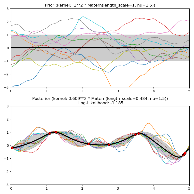
Illustration of prior and posterior Gaussian process for different kernels

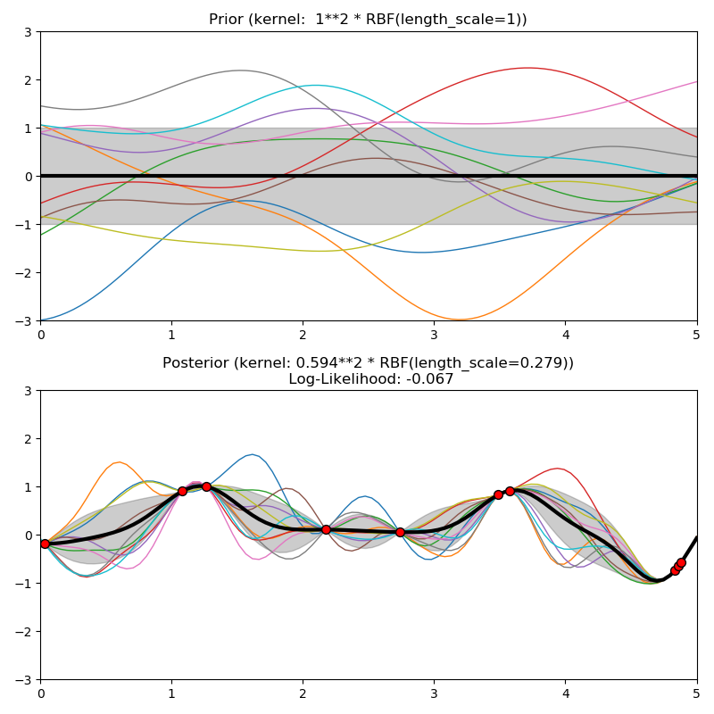
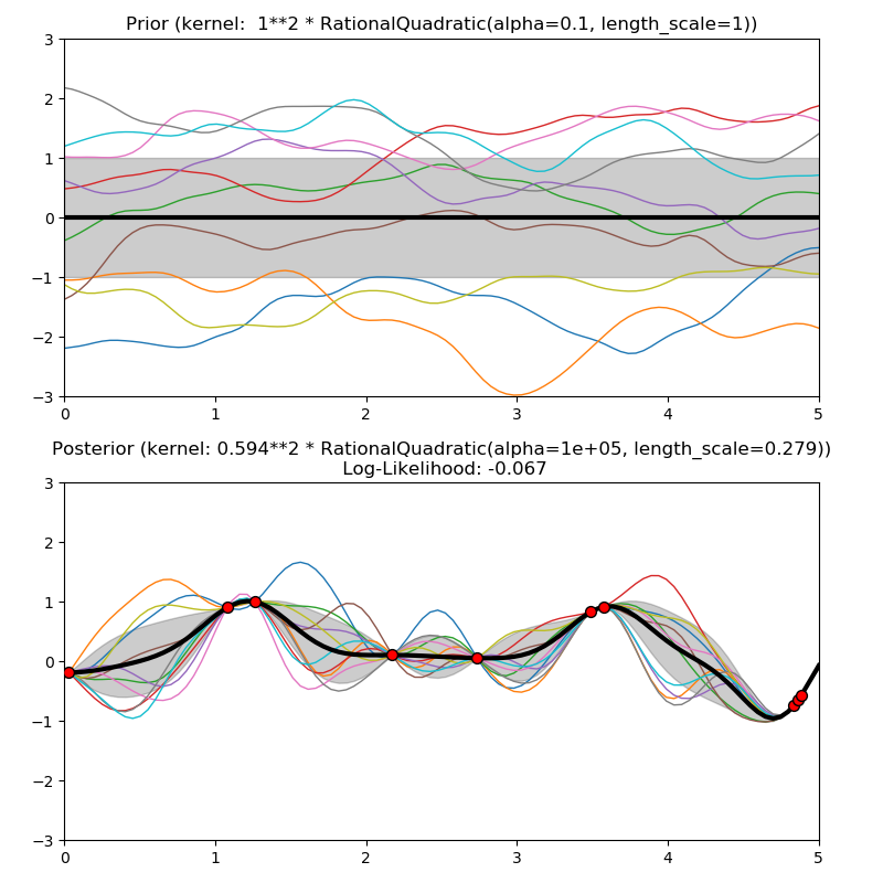
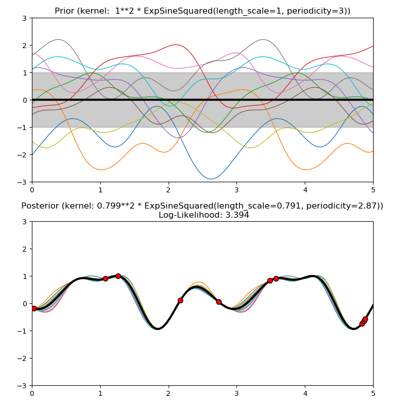
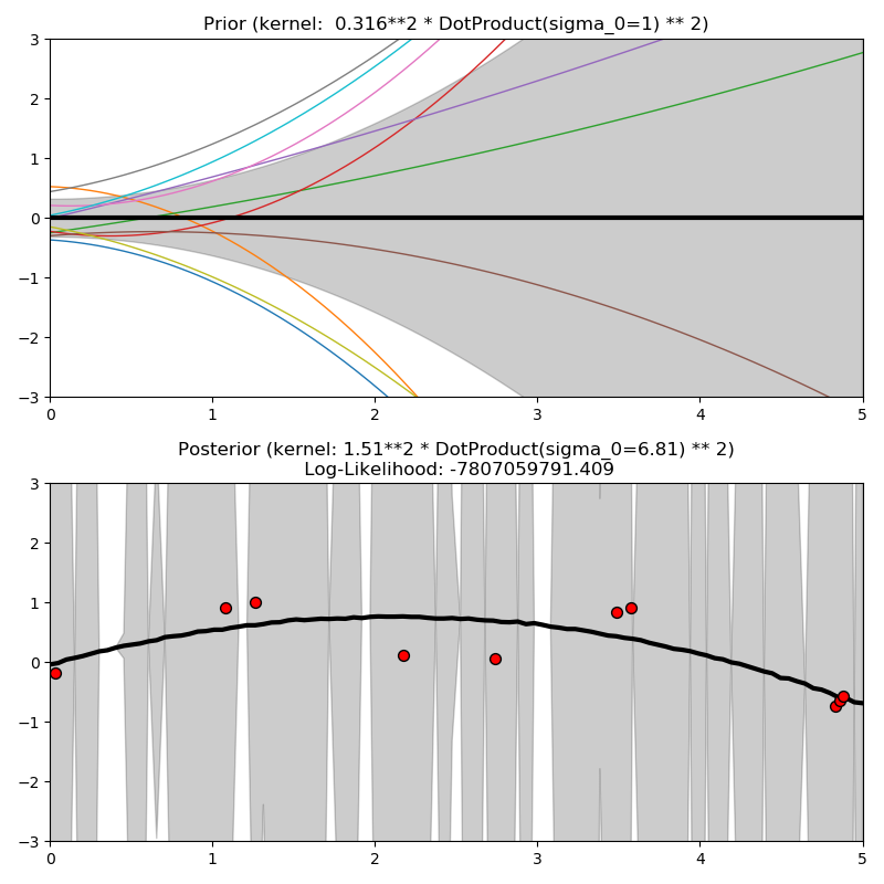
This example illustrates the prior and posterior of a GPR with different kernels. Mean, standard deviation, and 10 samples are shown for both prior and posterior.

• 
• 
• 
• 
• 

print(__doc__)

# Authors: Jan Hendrik Metzen <jhm@informatik.uni-bremen.de>
#
# License: BSD 3 clause

import numpy as np

from matplotlib import pyplot as plt

from sklearn.gaussian_process import GaussianProcessRegressor
from sklearn.gaussian_process.kernels import (RBF, Matern, RationalQuadratic,
                                              ExpSineSquared, DotProduct,
                                              ConstantKernel)


kernels = [1.0 * RBF(length_scale=1.0, length_scale_bounds=(1e-1, 10.0)),
           1.0 * RationalQuadratic(length_scale=1.0, alpha=0.1),
           1.0 * ExpSineSquared(length_scale=1.0, periodicity=3.0,
                                length_scale_bounds=(0.1, 10.0),
                                periodicity_bounds=(1.0, 10.0)),
           ConstantKernel(0.1, (0.01, 10.0))
               * (DotProduct(sigma_0=1.0, sigma_0_bounds=(0.0, 10.0)) ** 2),
           1.0 * Matern(length_scale=1.0, length_scale_bounds=(1e-1, 10.0),
                        nu=1.5)]

for fig_index, kernel in enumerate(kernels):
    # Specify Gaussian Process
    gp = GaussianProcessRegressor(kernel=kernel)

    # Plot prior
    plt.figure(fig_index, figsize=(8, 8))
    plt.subplot(2, 1, 1)
    X_ = np.linspace(0, 5, 100)
    y_mean, y_std = gp.predict(X_[:, np.newaxis], return_std=True)
    plt.plot(X_, y_mean, 'k', lw=3, zorder=9)
    plt.fill_between(X_, y_mean - y_std, y_mean + y_std,
                     alpha=0.2, color='k')
    y_samples = gp.sample_y(X_[:, np.newaxis], 10)
    plt.plot(X_, y_samples, lw=1)
    plt.xlim(0, 5)
    plt.ylim(-3, 3)
    plt.title("Prior (kernel:  %s)" % kernel, fontsize=12)

    # Generate data and fit GP
    rng = np.random.RandomState(4)
    X = rng.uniform(0, 5, 10)[:, np.newaxis]
    y = np.sin((X[:, 0] - 2.5) ** 2)
    gp.fit(X, y)

    # Plot posterior
    plt.subplot(2, 1, 2)
    X_ = np.linspace(0, 5, 100)
    y_mean, y_std = gp.predict(X_[:, np.newaxis], return_std=True)
    plt.plot(X_, y_mean, 'k', lw=3, zorder=9)
    plt.fill_between(X_, y_mean - y_std, y_mean + y_std,
                     alpha=0.2, color='k')

    y_samples = gp.sample_y(X_[:, np.newaxis], 10)
    plt.plot(X_, y_samples, lw=1)
    plt.scatter(X[:, 0], y, c='r', s=50, zorder=10, edgecolors=(0, 0, 0))
    plt.xlim(0, 5)
    plt.ylim(-3, 3)
    plt.title("Posterior (kernel: %s)\n Log-Likelihood: %.3f"
              % (gp.kernel_, gp.log_marginal_likelihood(gp.kernel_.theta)),
              fontsize=12)
    plt.tight_layout()

plt.show()

Total running time of the script: ( 0 minutes 1.138 seconds)