
3.3. Model evaluation: quantifying the quality of predictions
There are 3 different approaches to evaluate the quality of predictions of a model:
- Estimator score method: Estimators have a
scoremethod providing a default evaluation criterion for the problem they are designed to solve. This is not discussed on this page, but in each estimator’s documentation. - Scoring parameter: Model-evaluation tools using
cross-validation (such as
model_selection.cross_val_scoreandmodel_selection.GridSearchCV) rely on an internal scoring strategy. This is discussed in the section The scoring parameter: defining model evaluation rules. - Metric functions: The
metricsmodule implements functions assessing prediction error for specific purposes. These metrics are detailed in sections on Classification metrics, Multilabel ranking metrics, Regression metrics and Clustering metrics.
Finally, Dummy estimators are useful to get a baseline value of those metrics for random predictions.
See also
For “pairwise” metrics, between samples and not estimators or predictions, see the Pairwise metrics, Affinities and Kernels section.
3.3.1. The scoring parameter: defining model evaluation rules
Model selection and evaluation using tools, such as
model_selection.GridSearchCV and
model_selection.cross_val_score, take a scoring parameter that
controls what metric they apply to the estimators evaluated.
3.3.1.1. Common cases: predefined values
For the most common use cases, you can designate a scorer object with the
scoring parameter; the table below shows all possible values.
All scorer objects follow the convention that higher return values are better
than lower return values. Thus metrics which measure the distance between
the model and the data, like metrics.mean_squared_error, are
available as neg_mean_squared_error which return the negated value
of the metric.
| Scoring | Function | Comment |
|---|---|---|
| Classification | ||
| ‘accuracy’ | metrics.accuracy_score |
|
| ‘average_precision’ | metrics.average_precision_score |
|
| ‘f1’ | metrics.f1_score |
for binary targets |
| ‘f1_micro’ | metrics.f1_score |
micro-averaged |
| ‘f1_macro’ | metrics.f1_score |
macro-averaged |
| ‘f1_weighted’ | metrics.f1_score |
weighted average |
| ‘f1_samples’ | metrics.f1_score |
by multilabel sample |
| ‘neg_log_loss’ | metrics.log_loss |
requires predict_proba support |
| ‘precision’ etc. | metrics.precision_score |
suffixes apply as with ‘f1’ |
| ‘recall’ etc. | metrics.recall_score |
suffixes apply as with ‘f1’ |
| ‘roc_auc’ | metrics.roc_auc_score |
|
| Clustering | ||
| ‘adjusted_rand_score’ | metrics.adjusted_rand_score |
|
| Regression | ||
| ‘neg_mean_absolute_error’ | metrics.mean_absolute_error |
|
| ‘neg_mean_squared_error’ | metrics.mean_squared_error |
|
| ‘neg_median_absolute_error’ | metrics.median_absolute_error |
|
| ‘r2’ | metrics.r2_score |
Usage examples:
>>> from sklearn import svm, datasets
>>> from sklearn.model_selection import cross_val_score
>>> iris = datasets.load_iris()
>>> X, y = iris.data, iris.target
>>> clf = svm.SVC(probability=True, random_state=0)
>>> cross_val_score(clf, X, y, scoring='neg_log_loss')
array([-0.07..., -0.16..., -0.06...])
>>> model = svm.SVC()
>>> cross_val_score(model, X, y, scoring='wrong_choice')
Traceback (most recent call last):
ValueError: 'wrong_choice' is not a valid scoring value. Valid options are ['accuracy', 'adjusted_rand_score', 'average_precision', 'f1', 'f1_macro', 'f1_micro', 'f1_samples', 'f1_weighted', 'neg_log_loss', 'neg_mean_absolute_error', 'neg_mean_squared_error', 'neg_median_absolute_error', 'precision', 'precision_macro', 'precision_micro', 'precision_samples', 'precision_weighted', 'r2', 'recall', 'recall_macro', 'recall_micro', 'recall_samples', 'recall_weighted', 'roc_auc']
Note
The values listed by the ValueError exception correspond to the functions measuring
prediction accuracy described in the following sections.
The scorer objects for those functions are stored in the dictionary
sklearn.metrics.SCORERS.
3.3.1.2. Defining your scoring strategy from metric functions
The module sklearn.metric also exposes a set of simple functions
measuring a prediction error given ground truth and prediction:
- functions ending with
_scorereturn a value to maximize, the higher the better. - functions ending with
_erroror_lossreturn a value to minimize, the lower the better. When converting into a scorer object usingmake_scorer, set thegreater_is_betterparameter to False (True by default; see the parameter description below).
Metrics available for various machine learning tasks are detailed in sections below.
Many metrics are not given names to be used as scoring values,
sometimes because they require additional parameters, such as
fbeta_score. In such cases, you need to generate an appropriate
scoring object. The simplest way to generate a callable object for scoring
is by using make_scorer. That function converts metrics
into callables that can be used for model evaluation.
One typical use case is to wrap an existing metric function from the library
with non-default values for its parameters, such as the beta parameter for
the fbeta_score function:
>>> from sklearn.metrics import fbeta_score, make_scorer
>>> ftwo_scorer = make_scorer(fbeta_score, beta=2)
>>> from sklearn.model_selection import GridSearchCV
>>> from sklearn.svm import LinearSVC
>>> grid = GridSearchCV(LinearSVC(), param_grid={'C': [1, 10]}, scoring=ftwo_scorer)
The second use case is to build a completely custom scorer object
from a simple python function using make_scorer, which can
take several parameters:
- the python function you want to use (
my_custom_loss_funcin the example below) - whether the python function returns a score (
greater_is_better=True, the default) or a loss (greater_is_better=False). If a loss, the output of the python function is negated by the scorer object, conforming to the cross validation convention that scorers return higher values for better models. - for classification metrics only: whether the python function you provided requires continuous decision
certainties (
needs_threshold=True). The default value is False. - any additional parameters, such as
betaorlabelsinf1_score.
Here is an example of building custom scorers, and of using the
greater_is_better parameter:
>>> import numpy as np
>>> def my_custom_loss_func(ground_truth, predictions):
...     diff = np.abs(ground_truth - predictions).max()
...     return np.log(1 + diff)
...
>>> # loss_func will negate the return value of my_custom_loss_func,
>>> #  which will be np.log(2), 0.693, given the values for ground_truth
>>> #  and predictions defined below.
>>> loss  = make_scorer(my_custom_loss_func, greater_is_better=False)
>>> score = make_scorer(my_custom_loss_func, greater_is_better=True)
>>> ground_truth = [[1, 1]]
>>> predictions  = [0, 1]
>>> from sklearn.dummy import DummyClassifier
>>> clf = DummyClassifier(strategy='most_frequent', random_state=0)
>>> clf = clf.fit(ground_truth, predictions)
>>> loss(clf,ground_truth, predictions)
-0.69...
>>> score(clf,ground_truth, predictions)
0.69...
3.3.1.3. Implementing your own scoring object
You can generate even more flexible model scorers by constructing your own
scoring object from scratch, without using the make_scorer factory.
For a callable to be a scorer, it needs to meet the protocol specified by
the following two rules:
- It can be called with parameters
(estimator, X, y), whereestimatoris the model that should be evaluated,Xis validation data, andyis the ground truth target forX(in the supervised case) orNone(in the unsupervised case). - It returns a floating point number that quantifies the
estimatorprediction quality onX, with reference toy. Again, by convention higher numbers are better, so if your scorer returns loss, that value should be negated.
3.3.2. Classification metrics
The sklearn.metrics module implements several loss, score, and utility
functions to measure classification performance.
Some metrics might require probability estimates of the positive class,
confidence values, or binary decisions values.
Most implementations allow each sample to provide a weighted contribution
to the overall score, through the sample_weight parameter.
Some of these are restricted to the binary classification case:
matthews_corrcoef(y_true, y_pred[, ...]) |
Compute the Matthews correlation coefficient (MCC) for binary classes |
precision_recall_curve(y_true, probas_pred) |
Compute precision-recall pairs for different probability thresholds |
roc_curve(y_true, y_score[, pos_label, ...]) |
Compute Receiver operating characteristic (ROC) |
Others also work in the multiclass case:
cohen_kappa_score(y1, y2[, labels, weights]) |
Cohen’s kappa: a statistic that measures inter-annotator agreement. |
confusion_matrix(y_true, y_pred[, labels, ...]) |
Compute confusion matrix to evaluate the accuracy of a classification |
hinge_loss(y_true, pred_decision[, labels, ...]) |
Average hinge loss (non-regularized) |
Some also work in the multilabel case:
accuracy_score(y_true, y_pred[, normalize, ...]) |
Accuracy classification score. |
classification_report(y_true, y_pred[, ...]) |
Build a text report showing the main classification metrics |
f1_score(y_true, y_pred[, labels, ...]) |
Compute the F1 score, also known as balanced F-score or F-measure |
fbeta_score(y_true, y_pred, beta[, labels, ...]) |
Compute the F-beta score |
hamming_loss(y_true, y_pred[, labels, ...]) |
Compute the average Hamming loss. |
jaccard_similarity_score(y_true, y_pred[, ...]) |
Jaccard similarity coefficient score |
log_loss(y_true, y_pred[, eps, normalize, ...]) |
Log loss, aka logistic loss or cross-entropy loss. |
precision_recall_fscore_support(y_true, y_pred) |
Compute precision, recall, F-measure and support for each class |
precision_score(y_true, y_pred[, labels, ...]) |
Compute the precision |
recall_score(y_true, y_pred[, labels, ...]) |
Compute the recall |
zero_one_loss(y_true, y_pred[, normalize, ...]) |
Zero-one classification loss. |
And some work with binary and multilabel (but not multiclass) problems:
average_precision_score(y_true, y_score[, ...]) |
Compute average precision (AP) from prediction scores |
roc_auc_score(y_true, y_score[, average, ...]) |
Compute Area Under the Curve (AUC) from prediction scores |
In the following sub-sections, we will describe each of those functions, preceded by some notes on common API and metric definition.
3.3.2.1. From binary to multiclass and multilabel
Some metrics are essentially defined for binary classification tasks (e.g.
f1_score, roc_auc_score). In these cases, by default
only the positive label is evaluated, assuming by default that the positive
class is labelled 1 (though this may be configurable through the
pos_label parameter).
In extending a binary metric to multiclass or multilabel problems, the data
is treated as a collection of binary problems, one for each class.
There are then a number of ways to average binary metric calculations across
the set of classes, each of which may be useful in some scenario.
Where available, you should select among these using the average parameter.
"macro"simply calculates the mean of the binary metrics, giving equal weight to each class. In problems where infrequent classes are nonetheless important, macro-averaging may be a means of highlighting their performance. On the other hand, the assumption that all classes are equally important is often untrue, such that macro-averaging will over-emphasize the typically low performance on an infrequent class."weighted"accounts for class imbalance by computing the average of binary metrics in which each class’s score is weighted by its presence in the true data sample."micro"gives each sample-class pair an equal contribution to the overall metric (except as a result of sample-weight). Rather than summing the metric per class, this sums the dividends and divisors that make up the per-class metrics to calculate an overall quotient. Micro-averaging may be preferred in multilabel settings, including multiclass classification where a majority class is to be ignored."samples"applies only to multilabel problems. It does not calculate a per-class measure, instead calculating the metric over the true and predicted classes for each sample in the evaluation data, and returning their (sample_weight-weighted) average.- Selecting
average=Nonewill return an array with the score for each class.
While multiclass data is provided to the metric, like binary targets, as an
array of class labels, multilabel data is specified as an indicator matrix,
in which cell [i, j] has value 1 if sample i has label j and value
0 otherwise.
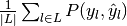
3.3.2.2. Accuracy score
The accuracy_score function computes the
accuracy, either the fraction
(default) or the count (normalize=False) of correct predictions.
In multilabel classification, the function returns the subset accuracy. If the entire set of predicted labels for a sample strictly match with the true set of labels, then the subset accuracy is 1.0; otherwise it is 0.0.
If  is the predicted value of
the
is the predicted value of
the  -th sample and
  is the corresponding true value,
then the fraction of correct predictions over
is the corresponding true value,
then the fraction of correct predictions over  is
defined as
is
defined as
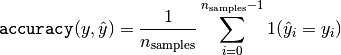
where  is the indicator function.
>>> import numpy as np
>>> from sklearn.metrics import accuracy_score
>>> y_pred = [0, 2, 1, 3]
>>> y_true = [0, 1, 2, 3]
>>> accuracy_score(y_true, y_pred)
0.5
>>> accuracy_score(y_true, y_pred, normalize=False)
2
In the multilabel case with binary label indicators:
>>> accuracy_score(np.array([[0, 1], [1, 1]]), np.ones((2, 2)))
0.5
Example:
- See Test with permutations the significance of a classification score for an example of accuracy score usage using permutations of the dataset.
3.3.2.3. Cohen’s kappa
The function cohen_kappa_score computes Cohen’s kappa statistic.
This measure is intended to compare labelings by different human annotators,
not a classifier versus a ground truth.
The kappa score (see docstring) is a number between -1 and 1. Scores above .8 are generally considered good agreement; zero or lower means no agreement (practically random labels).
Kappa scores can be computed for binary or multiclass problems, but not for multilabel problems (except by manually computing a per-label score) and not for more than two annotators.
>>> from sklearn.metrics import cohen_kappa_score
>>> y_true = [2, 0, 2, 2, 0, 1]
>>> y_pred = [0, 0, 2, 2, 0, 2]
>>> cohen_kappa_score(y_true, y_pred)
0.4285714285714286
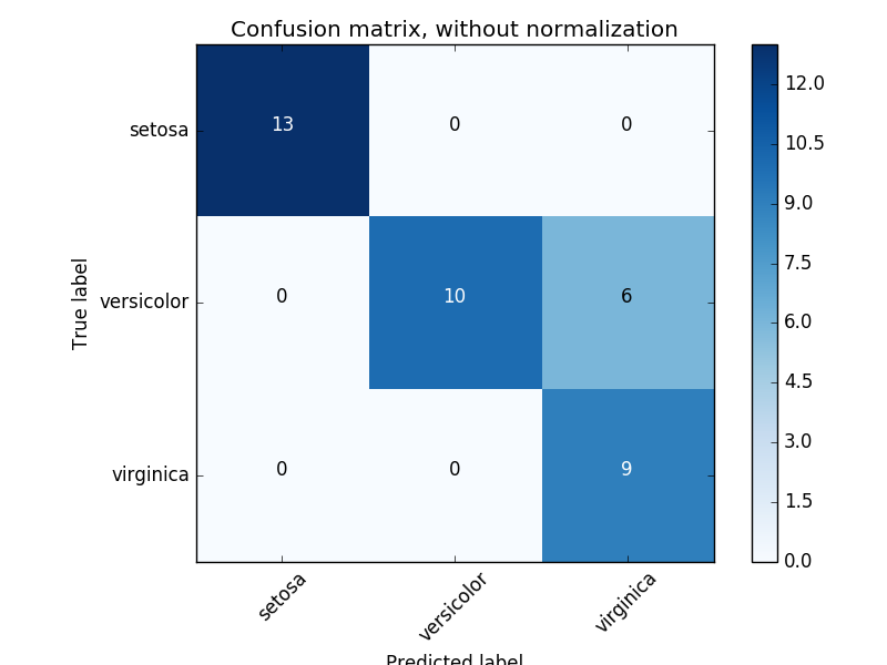
3.3.2.4. Confusion matrix
The confusion_matrix function evaluates
classification accuracy by computing the confusion matrix.
By definition, entry  in a confusion matrix is
the number of observations actually in group , but
predicted to be in group
in a confusion matrix is
the number of observations actually in group , but
predicted to be in group  . Here is an example:
>>> from sklearn.metrics import confusion_matrix
>>> y_true = [2, 0, 2, 2, 0, 1]
>>> y_pred = [0, 0, 2, 2, 0, 2]
>>> confusion_matrix(y_true, y_pred)
array([[2, 0, 0],
       [0, 0, 1],
       [1, 0, 2]])
Here is a visual representation of such a confusion matrix (this figure comes from the Confusion matrix example):
For binary problems, we can get counts of true negatives, false positives, false negatives and true positives as follows:
>>> y_true = [0, 0, 0, 1, 1, 1, 1, 1]
>>> y_pred = [0, 1, 0, 1, 0, 1, 0, 1]
>>> tn, fp, fn, tp = confusion_matrix(y_true, y_pred).ravel()
>>> tn, fp, fn, tp
(2, 1, 2, 3)
Example:
- See Confusion matrix for an example of using a confusion matrix to evaluate classifier output quality.
- See Recognizing hand-written digits for an example of using a confusion matrix to classify hand-written digits.
- See Classification of text documents using sparse features for an example of using a confusion matrix to classify text documents.
3.3.2.5. Classification report
The classification_report function builds a text report showing the
main classification metrics. Here is a small example with custom target_names
and inferred labels:
>>> from sklearn.metrics import classification_report
>>> y_true = [0, 1, 2, 2, 0]
>>> y_pred = [0, 0, 2, 1, 0]
>>> target_names = ['class 0', 'class 1', 'class 2']
>>> print(classification_report(y_true, y_pred, target_names=target_names))
             precision    recall  f1-score   support

    class 0       0.67      1.00      0.80         2
    class 1       0.00      0.00      0.00         1
    class 2       1.00      0.50      0.67         2

avg / total       0.67      0.60      0.59         5
Example:
- See Recognizing hand-written digits for an example of classification report usage for hand-written digits.
- See Classification of text documents using sparse features for an example of classification report usage for text documents.
- See Parameter estimation using grid search with cross-validation for an example of classification report usage for grid search with nested cross-validation.
3.3.2.6. Hamming loss
The hamming_loss computes the average Hamming loss or Hamming
distance between two sets
of samples.
If  is the predicted value for the -th label of
a given sample,
is the predicted value for the -th label of
a given sample,  is the corresponding true value, and
 is the number of classes or labels, then the
Hamming loss
is the number of classes or labels, then the
Hamming loss  between two samples is defined as:
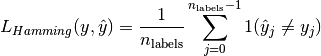
where is the indicator function.
>>> from sklearn.metrics import hamming_loss
>>> y_pred = [1, 2, 3, 4]
>>> y_true = [2, 2, 3, 4]
>>> hamming_loss(y_true, y_pred)
0.25
In the multilabel case with binary label indicators:
>>> hamming_loss(np.array([[0, 1], [1, 1]]), np.zeros((2, 2)))
0.75
Note
In multiclass classification, the Hamming loss corresponds to the Hamming
distance between y_true and y_pred which is similar to the
Zero one loss function. However, while zero-one loss penalizes
prediction sets that do not strictly match true sets, the Hamming loss
penalizes individual labels. Thus the Hamming loss, upper bounded by the zero-one
loss, is always between zero and one, inclusive; and predicting a proper subset
or superset of the true labels will give a Hamming loss between
zero and one, exclusive.
3.3.2.7. Jaccard similarity coefficient score
The jaccard_similarity_score function computes the average (default)
or sum of Jaccard similarity coefficients, also called the Jaccard index,
between pairs of label sets.
The Jaccard similarity coefficient of the -th samples,
with a ground truth label set and predicted label set
, is defined as
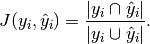
In binary and multiclass classification, the Jaccard similarity coefficient score is equal to the classification accuracy.
>>> import numpy as np
>>> from sklearn.metrics import jaccard_similarity_score
>>> y_pred = [0, 2, 1, 3]
>>> y_true = [0, 1, 2, 3]
>>> jaccard_similarity_score(y_true, y_pred)
0.5
>>> jaccard_similarity_score(y_true, y_pred, normalize=False)
2
In the multilabel case with binary label indicators:
>>> jaccard_similarity_score(np.array([[0, 1], [1, 1]]), np.ones((2, 2)))
0.75
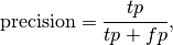
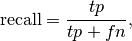
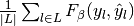
3.3.2.8. Precision, recall and F-measures
Intuitively, precision is the ability of the classifier not to label as positive a sample that is negative, and recall is the ability of the classifier to find all the positive samples.
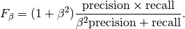
The F-measure
( and
and  measures) can be interpreted as a weighted
harmonic mean of the precision and recall. A
measure reaches its best value at 1 and its worst score at 0.
With
measures) can be interpreted as a weighted
harmonic mean of the precision and recall. A
measure reaches its best value at 1 and its worst score at 0.
With  , and
are equivalent, and the recall and the precision are equally important.
, and
are equivalent, and the recall and the precision are equally important.
The precision_recall_curve computes a precision-recall curve
from the ground truth label and a score given by the classifier
by varying a decision threshold.
The average_precision_score function computes the average precision
(AP) from prediction scores. This score corresponds to the area under the
precision-recall curve. The value is between 0 and 1 and higher is better.
With random predictions, the AP is the fraction of positive samples.
Several functions allow you to analyze the precision, recall and F-measures score:
average_precision_score(y_true, y_score[, ...]) |
Compute average precision (AP) from prediction scores |
f1_score(y_true, y_pred[, labels, ...]) |
Compute the F1 score, also known as balanced F-score or F-measure |
fbeta_score(y_true, y_pred, beta[, labels, ...]) |
Compute the F-beta score |
precision_recall_curve(y_true, probas_pred) |
Compute precision-recall pairs for different probability thresholds |
precision_recall_fscore_support(y_true, y_pred) |
Compute precision, recall, F-measure and support for each class |
precision_score(y_true, y_pred[, labels, ...]) |
Compute the precision |
recall_score(y_true, y_pred[, labels, ...]) |
Compute the recall |
Note that the precision_recall_curve function is restricted to the
binary case. The average_precision_score function works only in
binary classification and multilabel indicator format.
Examples:
- See Classification of text documents using sparse features
for an example of
f1_scoreusage to classify text documents. - See Parameter estimation using grid search with cross-validation
for an example of
precision_scoreandrecall_scoreusage to estimate parameters using grid search with nested cross-validation. - See Precision-Recall
for an example of
precision_recall_curveusage to evaluate classifier output quality. - See Sparse recovery: feature selection for sparse linear models
for an example of
precision_recall_curveusage to select features for sparse linear models.
3.3.2.8.1. Binary classification
In a binary classification task, the terms ‘’positive’’ and ‘’negative’’ refer to the classifier’s prediction, and the terms ‘’true’’ and ‘’false’’ refer to whether that prediction corresponds to the external judgment (sometimes known as the ‘’observation’‘). Given these definitions, we can formulate the following table:
| Actual class (observation) | ||
| Predicted class (expectation) | tp (true positive) Correct result | fp (false positive) Unexpected result |
| fn (false negative) Missing result | tn (true negative) Correct absence of result | |
In this context, we can define the notions of precision, recall and F-measure:
Here are some small examples in binary classification:
>>> from sklearn import metrics
>>> y_pred = [0, 1, 0, 0]
>>> y_true = [0, 1, 0, 1]
>>> metrics.precision_score(y_true, y_pred)
1.0
>>> metrics.recall_score(y_true, y_pred)
0.5
>>> metrics.f1_score(y_true, y_pred)
0.66...
>>> metrics.fbeta_score(y_true, y_pred, beta=0.5)
0.83...
>>> metrics.fbeta_score(y_true, y_pred, beta=1)
0.66...
>>> metrics.fbeta_score(y_true, y_pred, beta=2)
0.55...
>>> metrics.precision_recall_fscore_support(y_true, y_pred, beta=0.5)
(array([ 0.66...,  1.        ]), array([ 1. ,  0.5]), array([ 0.71...,  0.83...]), array([2, 2]...))


>>> import numpy as np
>>> from sklearn.metrics import precision_recall_curve
>>> from sklearn.metrics import average_precision_score
>>> y_true = np.array([0, 0, 1, 1])
>>> y_scores = np.array([0.1, 0.4, 0.35, 0.8])
>>> precision, recall, threshold = precision_recall_curve(y_true, y_scores)
>>> precision
array([ 0.66...,  0.5       ,  1.        ,  1.        ])
>>> recall
array([ 1. ,  0.5,  0.5,  0. ])
>>> threshold
array([ 0.35,  0.4 ,  0.8 ])
>>> average_precision_score(y_true, y_scores)
0.79...
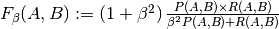
3.3.2.8.2. Multiclass and multilabel classification
In multiclass and multilabel classification task, the notions of precision,
recall, and F-measures can be applied to each label independently.
There are a few ways to combine results across labels,
specified by the average argument to the
average_precision_score (multilabel only), f1_score,
fbeta_score, precision_recall_fscore_support,
precision_score and recall_score functions, as described
above. Note that for “micro”-averaging in a multiclass setting
with all labels included will produce equal precision, recall and  ,
while “weighted” averaging may produce an F-score that is not between
precision and recall.
,
while “weighted” averaging may produce an F-score that is not between
precision and recall.
To make this more explicit, consider the following notation:
 the set of predicted
  pairs
pairs the set of true pairs
 the set of labels
 the set of samples
 the subset of with sample
  ,
i.e.
,
i.e. 
 the subset of with label
- similarly,
 and
and  are subsets of
 (Conventions vary on handling
  ; this implementation uses
 , and similar for
  .)
.)
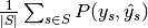
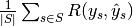
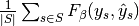
Then the metrics are defined as:
average |
Precision | Recall | F_beta |
|---|---|---|---|
"micro" |
 |
 |
 |
"samples" |
 |
 |
 |
"macro" |
 |
 |
 |
"weighted" |
 |
 |
 |
None |
 |
 |
 |
>>> from sklearn import metrics
>>> y_true = [0, 1, 2, 0, 1, 2]
>>> y_pred = [0, 2, 1, 0, 0, 1]
>>> metrics.precision_score(y_true, y_pred, average='macro')
0.22...
>>> metrics.recall_score(y_true, y_pred, average='micro')
...
0.33...
>>> metrics.f1_score(y_true, y_pred, average='weighted')
0.26...
>>> metrics.fbeta_score(y_true, y_pred, average='macro', beta=0.5)
0.23...
>>> metrics.precision_recall_fscore_support(y_true, y_pred, beta=0.5, average=None)
...
(array([ 0.66...,  0.        ,  0.        ]), array([ 1.,  0.,  0.]), array([ 0.71...,  0.        ,  0.        ]), array([2, 2, 2]...))
For multiclass classification with a “negative class”, it is possible to exclude some labels:
>>> metrics.recall_score(y_true, y_pred, labels=[1, 2], average='micro')
... # excluding 0, no labels were correctly recalled
0.0
Similarly, labels not present in the data sample may be accounted for in macro-averaging.
>>> metrics.precision_score(y_true, y_pred, labels=[0, 1, 2, 3], average='macro')
...
0.166...
3.3.2.9. Hinge loss
The hinge_loss function computes the average distance between
the model and the data using
hinge loss, a one-sided metric
that considers only prediction errors. (Hinge
loss is used in maximal margin classifiers such as support vector machines.)
If the labels are encoded with +1 and -1, : is the true
value, and  is the predicted decisions as output by
decision_function, then the hinge loss is defined as:

If there are more than two labels, hinge_loss uses a multiclass variant
due to Crammer & Singer.
Here is
the paper describing it.
If  is the predicted decision for true label and
  is the
maximum of the predicted decisions for all other labels, where predicted
decisions are output by decision function, then multiclass hinge loss is defined
by:
is the
maximum of the predicted decisions for all other labels, where predicted
decisions are output by decision function, then multiclass hinge loss is defined
by:

Here a small example demonstrating the use of the hinge_loss function
with a svm classifier in a binary class problem:
>>> from sklearn import svm
>>> from sklearn.metrics import hinge_loss
>>> X = [[0], [1]]
>>> y = [-1, 1]
>>> est = svm.LinearSVC(random_state=0)
>>> est.fit(X, y)
LinearSVC(C=1.0, class_weight=None, dual=True, fit_intercept=True,
     intercept_scaling=1, loss='squared_hinge', max_iter=1000,
     multi_class='ovr', penalty='l2', random_state=0, tol=0.0001,
     verbose=0)
>>> pred_decision = est.decision_function([[-2], [3], [0.5]])
>>> pred_decision
array([-2.18...,  2.36...,  0.09...])
>>> hinge_loss([-1, 1, 1], pred_decision)
0.3...
Here is an example demonstrating the use of the hinge_loss function
with a svm classifier in a multiclass problem:
>>> X = np.array([[0], [1], [2], [3]])
>>> Y = np.array([0, 1, 2, 3])
>>> labels = np.array([0, 1, 2, 3])
>>> est = svm.LinearSVC()
>>> est.fit(X, Y)
LinearSVC(C=1.0, class_weight=None, dual=True, fit_intercept=True,
     intercept_scaling=1, loss='squared_hinge', max_iter=1000,
     multi_class='ovr', penalty='l2', random_state=None, tol=0.0001,
     verbose=0)
>>> pred_decision = est.decision_function([[-1], [2], [3]])
>>> y_true = [0, 2, 3]
>>> hinge_loss(y_true, pred_decision, labels)
0.56...
3.3.2.10. Log loss
Log loss, also called logistic regression loss or
cross-entropy loss, is defined on probability estimates. It is
commonly used in (multinomial) logistic regression and neural networks, as well
as in some variants of expectation-maximization, and can be used to evaluate the
probability outputs (predict_proba) of a classifier instead of its
discrete predictions.
For binary classification with a true label  and a probability estimate
  ,
the log loss per sample is the negative log-likelihood
of the classifier given the true label:
,
the log loss per sample is the negative log-likelihood
of the classifier given the true label:

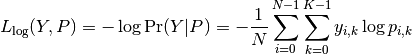
This extends to the multiclass case as follows.
Let the true labels for a set of samples
be encoded as a 1-of-K binary indicator matrix  ,
i.e.,
,
i.e.,  if sample has label
  taken from a set of
  labels.
Let be a matrix of probability estimates,
with
labels.
Let be a matrix of probability estimates,
with  .
Then the log loss of the whole set is
.
Then the log loss of the whole set is
To see how this generalizes the binary log loss given above,
note that in the binary case,
 and
and  ,
so expanding the inner sum over
,
so expanding the inner sum over  gives the binary log loss.
The log_loss function computes log loss given a list of ground-truth
labels and a probability matrix, as returned by an estimator’s predict_proba
method.
>>> from sklearn.metrics import log_loss
>>> y_true = [0, 0, 1, 1]
>>> y_pred = [[.9, .1], [.8, .2], [.3, .7], [.01, .99]]
>>> log_loss(y_true, y_pred)
0.1738...
The first [.9, .1] in y_pred denotes 90% probability that the first
sample has label 0. The log loss is non-negative.
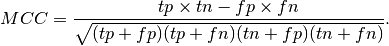
3.3.2.11. Matthews correlation coefficient
The matthews_corrcoef function computes the
Matthew’s correlation coefficient (MCC)
for binary classes. Quoting Wikipedia:
“The Matthews correlation coefficient is used in machine learning as a measure of the quality of binary (two-class) classifications. It takes into account true and false positives and negatives and is generally regarded as a balanced measure which can be used even if the classes are of very different sizes. The MCC is in essence a correlation coefficient value between -1 and +1. A coefficient of +1 represents a perfect prediction, 0 an average random prediction and -1 an inverse prediction. The statistic is also known as the phi coefficient.”
If  ,
,  ,
,  and
and  are respectively the
number of true positives, true negatives, false positives and false negatives,
the MCC coefficient is defined as
are respectively the
number of true positives, true negatives, false positives and false negatives,
the MCC coefficient is defined as
Here is a small example illustrating the usage of the matthews_corrcoef
function:
>>> from sklearn.metrics import matthews_corrcoef
>>> y_true = [+1, +1, +1, -1]
>>> y_pred = [+1, -1, +1, +1]
>>> matthews_corrcoef(y_true, y_pred)
-0.33...
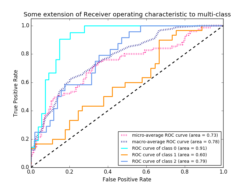
3.3.2.12. Receiver operating characteristic (ROC)
The function roc_curve computes the
receiver operating characteristic curve, or ROC curve.
Quoting Wikipedia :
“A receiver operating characteristic (ROC), or simply ROC curve, is a graphical plot which illustrates the performance of a binary classifier system as its discrimination threshold is varied. It is created by plotting the fraction of true positives out of the positives (TPR = true positive rate) vs. the fraction of false positives out of the negatives (FPR = false positive rate), at various threshold settings. TPR is also known as sensitivity, and FPR is one minus the specificity or true negative rate.”
This function requires the true binary
value and the target scores, which can either be probability estimates of the
positive class, confidence values, or binary decisions.
Here is a small example of how to use the roc_curve function:
>>> import numpy as np
>>> from sklearn.metrics import roc_curve
>>> y = np.array([1, 1, 2, 2])
>>> scores = np.array([0.1, 0.4, 0.35, 0.8])
>>> fpr, tpr, thresholds = roc_curve(y, scores, pos_label=2)
>>> fpr
array([ 0. ,  0.5,  0.5,  1. ])
>>> tpr
array([ 0.5,  0.5,  1. ,  1. ])
>>> thresholds
array([ 0.8 ,  0.4 ,  0.35,  0.1 ])
This figure shows an example of such an ROC curve:
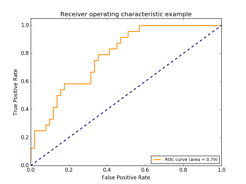
The roc_auc_score function computes the area under the receiver
operating characteristic (ROC) curve, which is also denoted by
AUC or AUROC. By computing the
area under the roc curve, the curve information is summarized in one number.
For more information see the Wikipedia article on AUC.
>>> import numpy as np
>>> from sklearn.metrics import roc_auc_score
>>> y_true = np.array([0, 0, 1, 1])
>>> y_scores = np.array([0.1, 0.4, 0.35, 0.8])
>>> roc_auc_score(y_true, y_scores)
0.75
In multi-label classification, the roc_auc_score function is
extended by averaging over the labels as above.
Compared to metrics such as the subset accuracy, the Hamming loss, or the
F1 score, ROC doesn’t require optimizing a threshold for each label. The
roc_auc_score function can also be used in multi-class classification,
if the predicted outputs have been binarized.
Examples:
- See Receiver Operating Characteristic (ROC) for an example of using ROC to evaluate the quality of the output of a classifier.
- See Receiver Operating Characteristic (ROC) with cross validation for an example of using ROC to evaluate classifier output quality, using cross-validation.
- See Species distribution modeling for an example of using ROC to model species distribution.
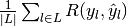
3.3.2.13. Zero one loss
The zero_one_loss function computes the sum or the average of the 0-1
classification loss ( ) over
  . By
default, the function normalizes over the sample. To get the sum of the
, set
. By
default, the function normalizes over the sample. To get the sum of the
, set normalize to False.
In multilabel classification, the zero_one_loss scores a subset as
one if its labels strictly match the predictions, and as a zero if there
are any errors. By default, the function returns the percentage of imperfectly
predicted subsets. To get the count of such subsets instead, set
normalize to False
If is the predicted value of
the -th sample and is the corresponding true value,
then the 0-1 loss is defined as:

where is the indicator function.
>>> from sklearn.metrics import zero_one_loss
>>> y_pred = [1, 2, 3, 4]
>>> y_true = [2, 2, 3, 4]
>>> zero_one_loss(y_true, y_pred)
0.25
>>> zero_one_loss(y_true, y_pred, normalize=False)
1
In the multilabel case with binary label indicators, where the first label set [0,1] has an error:
>>> zero_one_loss(np.array([[0, 1], [1, 1]]), np.ones((2, 2)))
0.5

>>> zero_one_loss(np.array([[0, 1], [1, 1]]), np.ones((2, 2)),  normalize=False)
1
Example:
- See Recursive feature elimination with cross-validation for an example of zero one loss usage to perform recursive feature elimination with cross-validation.
3.3.2.14. Brier score loss
The brier_score_loss function computes the
Brier score
for binary classes. Quoting Wikipedia:
“The Brier score is a proper score function that measures the accuracy of probabilistic predictions. It is applicable to tasks in which predictions must assign probabilities to a set of mutually exclusive discrete outcomes.”
This function returns a score of the mean square difference between the actual outcome and the predicted probability of the possible outcome. The actual outcome has to be 1 or 0 (true or false), while the predicted probability of the actual outcome can be a value between 0 and 1.
The brier score loss is also between 0 to 1 and the lower the score (the mean square difference is smaller), the more accurate the prediction is. It can be thought of as a measure of the “calibration” of a set of probabilistic predictions.
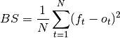
where :  is the total number of predictions,
  is the
predicted probablity of the actual outcome
is the
predicted probablity of the actual outcome  .
.
Here is a small example of usage of this function::
>>> import numpy as np
>>> from sklearn.metrics import brier_score_loss
>>> y_true = np.array([0, 1, 1, 0])
>>> y_true_categorical = np.array(["spam", "ham", "ham", "spam"])
>>> y_prob = np.array([0.1, 0.9, 0.8, 0.4])
>>> y_pred = np.array([0, 1, 1, 0])
>>> brier_score_loss(y_true, y_prob)
0.055
>>> brier_score_loss(y_true, 1-y_prob, pos_label=0)
0.055
>>> brier_score_loss(y_true_categorical, y_prob, pos_label="ham")
0.055
>>> brier_score_loss(y_true, y_prob > 0.5)
0.0
Example:
- See Probability calibration of classifiers for an example of Brier score loss usage to perform probability calibration of classifiers.
References:
- G. Brier, Verification of forecasts expressed in terms of probability, Monthly weather review 78.1 (1950)
3.3.3. Multilabel ranking metrics
In multilabel learning, each sample can have any number of ground truth labels associated with it. The goal is to give high scores and better rank to the ground truth labels.
3.3.3.1. Coverage error
The coverage_error function computes the average number of labels that
have to be included in the final prediction such that all true labels
are predicted. This is useful if you want to know how many top-scored-labels
you have to predict in average without missing any true one. The best value
of this metrics is thus the average number of true labels.
Formally, given a binary indicator matrix of the ground truth labels
 and the
score associated with each label
and the
score associated with each label
 ,
the coverage is defined as
,
the coverage is defined as
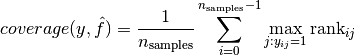
with 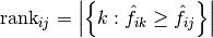 .
Given the rank definition, ties in
.
Given the rank definition, ties in y_scores are broken by giving the
maximal rank that would have been assigned to all tied values.
Here is a small example of usage of this function:
>>> import numpy as np
>>> from sklearn.metrics import coverage_error
>>> y_true = np.array([[1, 0, 0], [0, 0, 1]])
>>> y_score = np.array([[0.75, 0.5, 1], [1, 0.2, 0.1]])
>>> coverage_error(y_true, y_score)
2.5
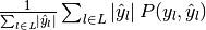
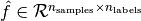
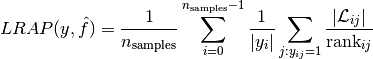
3.3.3.2. Label ranking average precision
The label_ranking_average_precision_score function
implements label ranking average precision (LRAP). This metric is linked to
the average_precision_score function, but is based on the notion of
label ranking instead of precision and recall.
Label ranking average precision (LRAP) is the average over each ground truth label assigned to each sample, of the ratio of true vs. total labels with lower score. This metric will yield better scores if you are able to give better rank to the labels associated with each sample. The obtained score is always strictly greater than 0, and the best value is 1. If there is exactly one relevant label per sample, label ranking average precision is equivalent to the mean reciprocal rank.
Formally, given a binary indicator matrix of the ground truth labels
 and the
score associated with each label
and the
score associated with each label
 ,
the average precision is defined as
,
the average precision is defined as
with 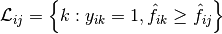 ,
and
,
and  is the l0 norm or the cardinality of the set.
Here is a small example of usage of this function:
>>> import numpy as np
>>> from sklearn.metrics import label_ranking_average_precision_score
>>> y_true = np.array([[1, 0, 0], [0, 0, 1]])
>>> y_score = np.array([[0.75, 0.5, 1], [1, 0.2, 0.1]])
>>> label_ranking_average_precision_score(y_true, y_score)
0.416...
3.3.3.3. Ranking loss
The label_ranking_loss function computes the ranking loss which
averages over the samples the number of label pairs that are incorrectly
ordered, i.e. true labels have a lower score than false labels, weighted by
the inverse number of false and true labels. The lowest achievable
ranking loss is zero.
Formally, given a binary indicator matrix of the ground truth labels
and the
score associated with each label
,
the ranking loss is defined as

where is the  norm or the cardinality of the set.
Here is a small example of usage of this function:
>>> import numpy as np
>>> from sklearn.metrics import label_ranking_loss
>>> y_true = np.array([[1, 0, 0], [0, 0, 1]])
>>> y_score = np.array([[0.75, 0.5, 1], [1, 0.2, 0.1]])
>>> label_ranking_loss(y_true, y_score)
0.75...
>>> # With the following prediction, we have perfect and minimal loss
>>> y_score = np.array([[1.0, 0.1, 0.2], [0.1, 0.2, 0.9]])
>>> label_ranking_loss(y_true, y_score)
0.0
3.3.4. Regression metrics
The sklearn.metrics module implements several loss, score, and utility
functions to measure regression performance. Some of those have been enhanced
to handle the multioutput case: mean_squared_error,
mean_absolute_error, explained_variance_score and
r2_score.
These functions have an multioutput keyword argument which specifies the
way the scores or losses for each individual target should be averaged. The
default is 'uniform_average', which specifies a uniformly weighted mean
over outputs. If an ndarray of shape (n_outputs,) is passed, then its
entries are interpreted as weights and an according weighted average is
returned. If multioutput is 'raw_values' is specified, then all
unaltered individual scores or losses will be returned in an array of shape
(n_outputs,).
The r2_score and explained_variance_score accept an additional
value 'variance_weighted' for the multioutput parameter. This option
leads to a weighting of each individual score by the variance of the
corresponding target variable. This setting quantifies the globally captured
unscaled variance. If the target variables are of different scale, then this
score puts more importance on well explaining the higher variance variables.
multioutput='variance_weighted' is the default value for r2_score
for backward compatibility. This will be changed to uniform_average in the
future.
3.3.4.1. Explained variance score
The explained_variance_score computes the explained variance
regression score.
If is the estimated target output, the corresponding
(correct) target output, and  is Variance, the square of the standard deviation,
then the explained variance is estimated as follow:
is Variance, the square of the standard deviation,
then the explained variance is estimated as follow:
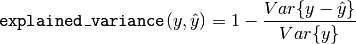
The best possible score is 1.0, lower values are worse.
Here is a small example of usage of the explained_variance_score
function:
>>> from sklearn.metrics import explained_variance_score
>>> y_true = [3, -0.5, 2, 7]
>>> y_pred = [2.5, 0.0, 2, 8]
>>> explained_variance_score(y_true, y_pred)
0.957...
>>> y_true = [[0.5, 1], [-1, 1], [7, -6]]
>>> y_pred = [[0, 2], [-1, 2], [8, -5]]
>>> explained_variance_score(y_true, y_pred, multioutput='raw_values')
...
array([ 0.967...,  1.        ])
>>> explained_variance_score(y_true, y_pred, multioutput=[0.3, 0.7])
...
0.990...
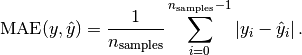
3.3.4.2. Mean absolute error
The mean_absolute_error function computes mean absolute
error, a risk
metric corresponding to the expected value of the absolute error loss or
 -norm loss.
If is the predicted value of the -th sample,
and is the corresponding true value, then the mean absolute error
(MAE) estimated over is defined as
Here is a small example of usage of the mean_absolute_error function:
>>> from sklearn.metrics import mean_absolute_error
>>> y_true = [3, -0.5, 2, 7]
>>> y_pred = [2.5, 0.0, 2, 8]
>>> mean_absolute_error(y_true, y_pred)
0.5
>>> y_true = [[0.5, 1], [-1, 1], [7, -6]]
>>> y_pred = [[0, 2], [-1, 2], [8, -5]]
>>> mean_absolute_error(y_true, y_pred)
0.75
>>> mean_absolute_error(y_true, y_pred, multioutput='raw_values')
array([ 0.5,  1. ])
>>> mean_absolute_error(y_true, y_pred, multioutput=[0.3, 0.7])
...
0.849...
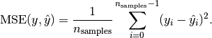
3.3.4.3. Mean squared error
The mean_squared_error function computes mean square
error, a risk
metric corresponding to the expected value of the squared (quadratic) error loss or
loss.
If is the predicted value of the -th sample,
and is the corresponding true value, then the mean squared error
(MSE) estimated over is defined as
Here is a small example of usage of the mean_squared_error
function:
>>> from sklearn.metrics import mean_squared_error
>>> y_true = [3, -0.5, 2, 7]
>>> y_pred = [2.5, 0.0, 2, 8]
>>> mean_squared_error(y_true, y_pred)
0.375
>>> y_true = [[0.5, 1], [-1, 1], [7, -6]]
>>> y_pred = [[0, 2], [-1, 2], [8, -5]]
>>> mean_squared_error(y_true, y_pred)
0.7083...
Examples:
- See Gradient Boosting regression for an example of mean squared error usage to evaluate gradient boosting regression.
3.3.4.4. Median absolute error
The median_absolute_error is particularly interesting because it is
robust to outliers. The loss is calculated by taking the median of all absolute
differences between the target and the prediction.
If is the predicted value of the -th sample
and is the corresponding true value, then the median absolute error
(MedAE) estimated over is defined as

The median_absolute_error does not support multioutput.
Here is a small example of usage of the median_absolute_error
function:
>>> from sklearn.metrics import median_absolute_error
>>> y_true = [3, -0.5, 2, 7]
>>> y_pred = [2.5, 0.0, 2, 8]
>>> median_absolute_error(y_true, y_pred)
0.5
3.3.4.5. R² score, the coefficient of determination
The r2_score function computes R², the coefficient of
determination.
It provides a measure of how well future samples are likely to
be predicted by the model. Best possible score is 1.0 and it can be negative
(because the model can be arbitrarily worse). A constant model that always
predicts the expected value of y, disregarding the input features, would get a
R^2 score of 0.0.
If is the predicted value of the -th sample
and is the corresponding true value, then the score R² estimated
over is defined as
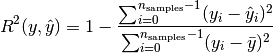
where 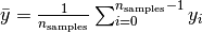 .
.
Here is a small example of usage of the r2_score function:
>>> from sklearn.metrics import r2_score
>>> y_true = [3, -0.5, 2, 7]
>>> y_pred = [2.5, 0.0, 2, 8]
>>> r2_score(y_true, y_pred)
0.948...
>>> y_true = [[0.5, 1], [-1, 1], [7, -6]]
>>> y_pred = [[0, 2], [-1, 2], [8, -5]]
>>> r2_score(y_true, y_pred, multioutput='variance_weighted')
...
0.938...
>>> y_true = [[0.5, 1], [-1, 1], [7, -6]]
>>> y_pred = [[0, 2], [-1, 2], [8, -5]]
>>> r2_score(y_true, y_pred, multioutput='uniform_average')
...
0.936...
>>> r2_score(y_true, y_pred, multioutput='raw_values')
...
array([ 0.965...,  0.908...])
>>> r2_score(y_true, y_pred, multioutput=[0.3, 0.7])
...
0.925...
Example:
- See Lasso and Elastic Net for Sparse Signals for an example of R² score usage to evaluate Lasso and Elastic Net on sparse signals.
3.3.5. Clustering metrics
The sklearn.metrics module implements several loss, score, and utility
functions. For more information see the Clustering performance evaluation
section for instance clustering, and Biclustering evaluation for
biclustering.
3.3.6. Dummy estimators
When doing supervised learning, a simple sanity check consists of comparing
one’s estimator against simple rules of thumb. DummyClassifier
implements several such simple strategies for classification:
stratifiedgenerates random predictions by respecting the training set class distribution.most_frequentalways predicts the most frequent label in the training set.prioralways predicts the class that maximizes the class prior (likemost_frequent`) and ``predict_probareturns the class prior.uniformgenerates predictions uniformly at random.constantalways predicts a constant label that is provided by the user.A major motivation of this method is F1-scoring, when the positive class is in the minority.
Note that with all these strategies, the predict method completely ignores
the input data!
To illustrate DummyClassifier, first let’s create an imbalanced
dataset:
>>> from sklearn.datasets import load_iris
>>> from sklearn.model_selection import train_test_split
>>> iris = load_iris()
>>> X, y = iris.data, iris.target
>>> y[y != 1] = -1
>>> X_train, X_test, y_train, y_test = train_test_split(X, y, random_state=0)
Next, let’s compare the accuracy of SVC and most_frequent:
>>> from sklearn.dummy import DummyClassifier
>>> from sklearn.svm import SVC
>>> clf = SVC(kernel='linear', C=1).fit(X_train, y_train)
>>> clf.score(X_test, y_test)
0.63...
>>> clf = DummyClassifier(strategy='most_frequent',random_state=0)
>>> clf.fit(X_train, y_train)
DummyClassifier(constant=None, random_state=0, strategy='most_frequent')
>>> clf.score(X_test, y_test)
0.57...
We see that SVC doesn’t do much better than a dummy classifier. Now, let’s
change the kernel:
>>> clf = SVC(kernel='rbf', C=1).fit(X_train, y_train)
>>> clf.score(X_test, y_test)
0.97...
We see that the accuracy was boosted to almost 100%. A cross validation strategy is recommended for a better estimate of the accuracy, if it is not too CPU costly. For more information see the Cross-validation: evaluating estimator performance section. Moreover if you want to optimize over the parameter space, it is highly recommended to use an appropriate methodology; see the Tuning the hyper-parameters of an estimator section for details.
More generally, when the accuracy of a classifier is too close to random, it probably means that something went wrong: features are not helpful, a hyperparameter is not correctly tuned, the classifier is suffering from class imbalance, etc...
DummyRegressor also implements four simple rules of thumb for regression:
meanalways predicts the mean of the training targets.medianalways predicts the median of the training targets.quantilealways predicts a user provided quantile of the training targets.constantalways predicts a constant value that is provided by the user.
In all these strategies, the predict method completely ignores
the input data.