Receiver Operating Characteristic (ROC) with cross validation

Example of Receiver Operating Characteristic (ROC) metric to evaluate classifier output quality using cross-validation.

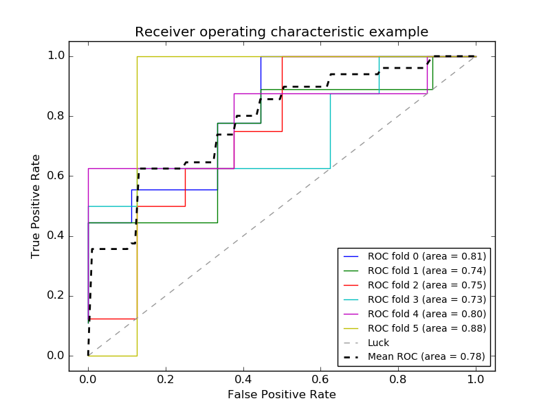
ROC curves typically feature true positive rate on the Y axis, and false positive rate on the X axis. This means that the top left corner of the plot is the “ideal” point - a false positive rate of zero, and a true positive rate of one. This is not very realistic, but it does mean that a larger area under the curve (AUC) is usually better.

The “steepness” of ROC curves is also important, since it is ideal to maximize the true positive rate while minimizing the false positive rate.

This example shows the ROC response of different datasets, created from K-fold cross-validation. Taking all of these curves, it is possible to calculate the mean area under curve, and see the variance of the curve when the training set is split into different subsets. This roughly shows how the classifier output is affected by changes in the training data, and how different the splits generated by K-fold cross-validation are from one another.

Note

See also sklearn.metrics.auc_score,

sklearn.cross_validation.cross_val_score, Receiver Operating Characteristic (ROC),

Python source code: plot_roc_crossval.py

print(__doc__)

import numpy as np
from scipy import interp
import matplotlib.pyplot as plt

from sklearn import svm, datasets
from sklearn.metrics import roc_curve, auc
from sklearn.cross_validation import StratifiedKFold

###############################################################################
# Data IO and generation

# import some data to play with
iris = datasets.load_iris()
X = iris.data
y = iris.target
X, y = X[y != 2], y[y != 2]
n_samples, n_features = X.shape

# Add noisy features
random_state = np.random.RandomState(0)
X = np.c_[X, random_state.randn(n_samples, 200 * n_features)]

###############################################################################
# Classification and ROC analysis

# Run classifier with cross-validation and plot ROC curves
cv = StratifiedKFold(y, n_folds=6)
classifier = svm.SVC(kernel='linear', probability=True,
                     random_state=random_state)

mean_tpr = 0.0
mean_fpr = np.linspace(0, 1, 100)
all_tpr = []

for i, (train, test) in enumerate(cv):
    probas_ = classifier.fit(X[train], y[train]).predict_proba(X[test])
    # Compute ROC curve and area the curve
    fpr, tpr, thresholds = roc_curve(y[test], probas_[:, 1])
    mean_tpr += interp(mean_fpr, fpr, tpr)
    mean_tpr[0] = 0.0
    roc_auc = auc(fpr, tpr)
    plt.plot(fpr, tpr, lw=1, label='ROC fold %d (area = %0.2f)' % (i, roc_auc))

plt.plot([0, 1], [0, 1], '--', color=(0.6, 0.6, 0.6), label='Luck')

mean_tpr /= len(cv)
mean_tpr[-1] = 1.0
mean_auc = auc(mean_fpr, mean_tpr)
plt.plot(mean_fpr, mean_tpr, 'k--',
         label='Mean ROC (area = %0.2f)' % mean_auc, lw=2)

plt.xlim([-0.05, 1.05])
plt.ylim([-0.05, 1.05])
plt.xlabel('False Positive Rate')
plt.ylabel('True Positive Rate')
plt.title('Receiver operating characteristic example')
plt.legend(loc="lower right")
plt.show()

Total running time of the example: 0.42 seconds ( 0 minutes 0.42 seconds)