Confusion matrix

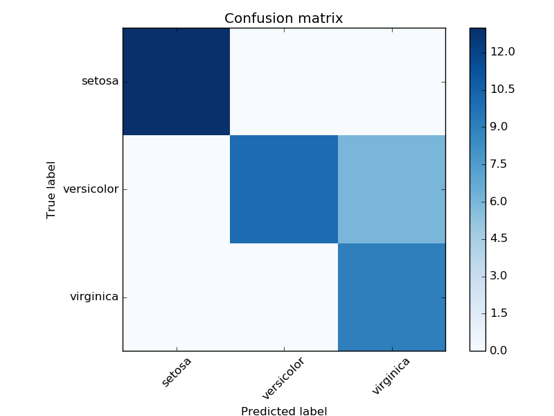
Example of confusion matrix usage to evaluate the quality of the output of a classifier on the iris data set. The diagonal elements represent the number of points for which the predicted label is equal to the true label, while off-diagonal elements are those that are mislabeled by the classifier. The higher the diagonal values of the confusion matrix the better, indicating many correct predictions.

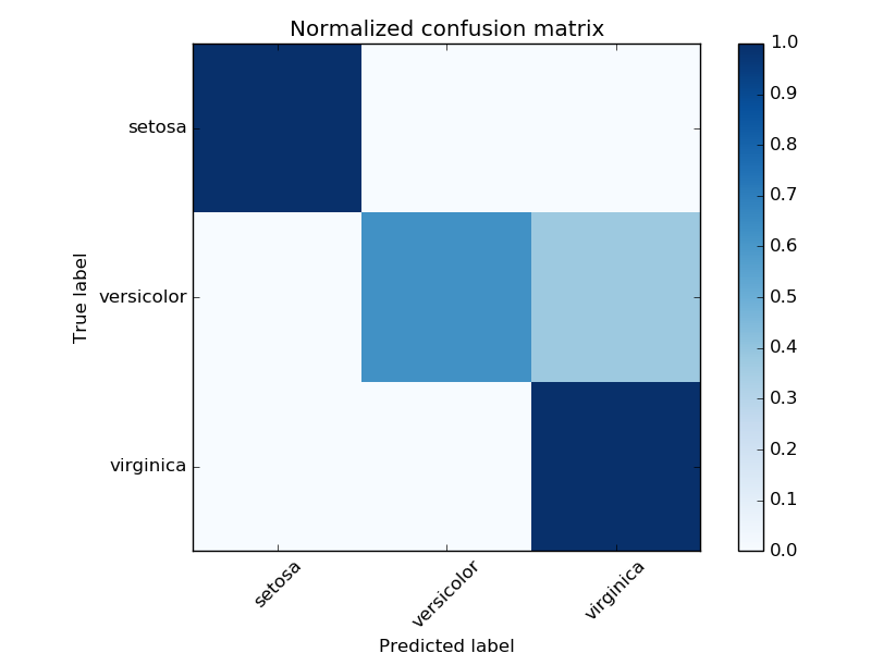
The figures show the confusion matrix with and without normalization by class support size (number of elements in each class). This kind of normalization can be interesting in case of class imbalance to have a more visual interpretation of which class is being misclassified.

Here the results are not as good as they could be as our choice for the regularization parameter C was not the best. In real life applications this parameter is usually chosen using Grid Search: Searching for estimator parameters.

• 
• 

Script output:

Confusion matrix, without normalization
[[13  0  0]
 [ 0 10  6]
 [ 0  0  9]]
Normalized confusion matrix
[[ 1.    0.    0.  ]
 [ 0.    0.62  0.38]
 [ 0.    0.    1.  ]]

Python source code: plot_confusion_matrix.py

print(__doc__)

import numpy as np
import matplotlib.pyplot as plt

from sklearn import svm, datasets
from sklearn.cross_validation import train_test_split
from sklearn.metrics import confusion_matrix

# import some data to play with
iris = datasets.load_iris()
X = iris.data
y = iris.target

# Split the data into a training set and a test set
X_train, X_test, y_train, y_test = train_test_split(X, y, random_state=0)

# Run classifier, using a model that is too regularized (C too low) to see
# the impact on the results
classifier = svm.SVC(kernel='linear', C=0.01)
y_pred = classifier.fit(X_train, y_train).predict(X_test)


def plot_confusion_matrix(cm, title='Confusion matrix', cmap=plt.cm.Blues):
    plt.imshow(cm, interpolation='nearest', cmap=cmap)
    plt.title(title)
    plt.colorbar()
    tick_marks = np.arange(len(iris.target_names))
    plt.xticks(tick_marks, iris.target_names, rotation=45)
    plt.yticks(tick_marks, iris.target_names)
    plt.tight_layout()
    plt.ylabel('True label')
    plt.xlabel('Predicted label')


# Compute confusion matrix
cm = confusion_matrix(y_test, y_pred)
np.set_printoptions(precision=2)
print('Confusion matrix, without normalization')
print(cm)
plt.figure()
plot_confusion_matrix(cm)

# Normalize the confusion matrix by row (i.e by the number of samples
# in each class)
cm_normalized = cm.astype('float') / cm.sum(axis=1)[:, np.newaxis]
print('Normalized confusion matrix')
print(cm_normalized)
plt.figure()
plot_confusion_matrix(cm_normalized, title='Normalized confusion matrix')

plt.show()

Total running time of the example: 0.44 seconds ( 0 minutes 0.44 seconds)