Hierarchical clustering: structured vs unstructured ward

Example builds a swiss roll dataset and runs hierarchical clustering on their position.

For more information, see Hierarchical clustering.

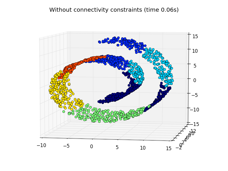
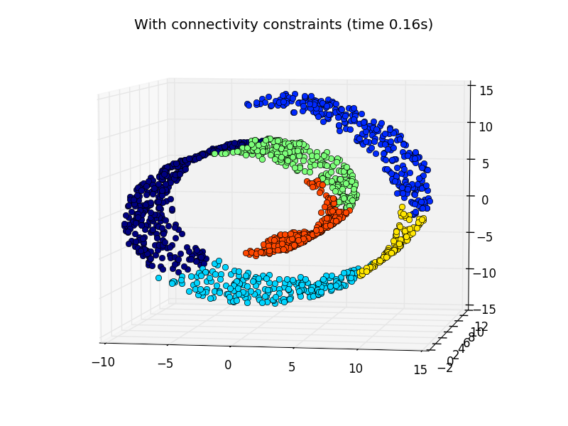
In a first step, the hierarchical clustering is performed without connectivity constraints on the structure and is solely based on distance, whereas in a second step the clustering is restricted to the k-Nearest Neighbors graph: it’s a hierarchical clustering with structure prior.

Some of the clusters learned without connectivity constraints do not respect the structure of the swiss roll and extend across different folds of the manifolds. On the opposite, when opposing connectivity constraints, the clusters form a nice parcellation of the swiss roll.

# Authors : Vincent Michel, 2010
#           Alexandre Gramfort, 2010
#           Gael Varoquaux, 2010
# License: BSD 3 clause

print(__doc__)

import time as time
import numpy as np
import matplotlib.pyplot as plt
import mpl_toolkits.mplot3d.axes3d as p3
from sklearn.cluster import AgglomerativeClustering
from sklearn.datasets.samples_generator import make_swiss_roll

Generate data (swiss roll dataset)

n_samples = 1500
noise = 0.05
X, _ = make_swiss_roll(n_samples, noise)
# Make it thinner
X[:, 1] *= .5

Compute clustering

print("Compute unstructured hierarchical clustering...")
st = time.time()
ward = AgglomerativeClustering(n_clusters=6, linkage='ward').fit(X)
elapsed_time = time.time() - st
label = ward.labels_
print("Elapsed time: %.2fs" % elapsed_time)
print("Number of points: %i" % label.size)

Out:

  Compute unstructured hierarchical clustering...
Elapsed time: 0.06s
Number of points: 1500

Plot result

fig = plt.figure()
ax = p3.Axes3D(fig)
ax.view_init(7, -80)
for l in np.unique(label):
    ax.plot3D(X[label == l, 0], X[label == l, 1], X[label == l, 2],
              'o', color=plt.cm.jet(np.float(l) / np.max(label + 1)))
plt.title('Without connectivity constraints (time %.2fs)' % elapsed_time)

Define the structure A of the data. Here a 10 nearest neighbors

from sklearn.neighbors import kneighbors_graph
connectivity = kneighbors_graph(X, n_neighbors=10, include_self=False)

Compute clustering

print("Compute structured hierarchical clustering...")
st = time.time()
ward = AgglomerativeClustering(n_clusters=6, connectivity=connectivity,
                               linkage='ward').fit(X)
elapsed_time = time.time() - st
label = ward.labels_
print("Elapsed time: %.2fs" % elapsed_time)
print("Number of points: %i" % label.size)

Out:

  Compute structured hierarchical clustering...
Elapsed time: 0.16s
Number of points: 1500

Plot result

fig = plt.figure()
ax = p3.Axes3D(fig)
ax.view_init(7, -80)
for l in np.unique(label):
    ax.plot3D(X[label == l, 0], X[label == l, 1], X[label == l, 2],
              'o', color=plt.cm.jet(float(l) / np.max(label + 1)))
plt.title('With connectivity constraints (time %.2fs)' % elapsed_time)

plt.show()

Total running time of the script: (0 minutes 0.317 seconds)

Download Python source code: plot_ward_structured_vs_unstructured.py

Download IPython notebook: plot_ward_structured_vs_unstructured.ipynb