Note
Go to the end to download the full example code or to run this example in your browser via JupyterLite or Binder
Clustering text documents using k-means
This is an example showing how the scikit-learn API can be used to cluster documents by topics using a Bag of Words approach.
Two algorithms are demonstrated, namely KMeans and its more
scalable variant, MiniBatchKMeans. Additionally,
latent semantic analysis is used to reduce dimensionality and discover latent
patterns in the data.
This example uses two different text vectorizers: a
TfidfVectorizer and a
HashingVectorizer. See the example
notebook FeatureHasher and DictVectorizer Comparison
for more information on vectorizers and a comparison of their processing times.
For document analysis via a supervised learning approach, see the example script Classification of text documents using sparse features.
# Author: Peter Prettenhofer <peter.prettenhofer@gmail.com>
#         Lars Buitinck
#         Olivier Grisel <olivier.grisel@ensta.org>
#         Arturo Amor <david-arturo.amor-quiroz@inria.fr>
# License: BSD 3 clause
Loading text data
We load data from The 20 newsgroups text dataset, which comprises around 18,000 newsgroups posts on 20 topics. For illustrative purposes and to reduce the computational cost, we select a subset of 4 topics only accounting for around 3,400 documents. See the example Classification of text documents using sparse features to gain intuition on the overlap of such topics.
Notice that, by default, the text samples contain some message metadata such
as "headers", "footers" (signatures) and "quotes" to other posts. We use
the remove parameter from fetch_20newsgroups to
strip those features and have a more sensible clustering problem.
import numpy as np

from sklearn.datasets import fetch_20newsgroups

categories = [
    "alt.atheism",
    "talk.religion.misc",
    "comp.graphics",
    "sci.space",
]

dataset = fetch_20newsgroups(
    remove=("headers", "footers", "quotes"),
    subset="all",
    categories=categories,
    shuffle=True,
    random_state=42,
)

labels = dataset.target
unique_labels, category_sizes = np.unique(labels, return_counts=True)
true_k = unique_labels.shape[0]

print(f"{len(dataset.data)} documents - {true_k} categories")
3387 documents - 4 categories
Quantifying the quality of clustering results
In this section we define a function to score different clustering pipelines using several metrics.
Clustering algorithms are fundamentally unsupervised learning methods. However, since we happen to have class labels for this specific dataset, it is possible to use evaluation metrics that leverage this “supervised” ground truth information to quantify the quality of the resulting clusters. Examples of such metrics are the following:
homogeneity, which quantifies how much clusters contain only members of a single class;
completeness, which quantifies how much members of a given class are assigned to the same clusters;
V-measure, the harmonic mean of completeness and homogeneity;
Rand-Index, which measures how frequently pairs of data points are grouped consistently according to the result of the clustering algorithm and the ground truth class assignment;
Adjusted Rand-Index, a chance-adjusted Rand-Index such that random cluster assignment have an ARI of 0.0 in expectation.
If the ground truth labels are not known, evaluation can only be performed using the model results itself. In that case, the Silhouette Coefficient comes in handy. See Selecting the number of clusters with silhouette analysis on KMeans clustering for an example on how to do it.
For more reference, see Clustering performance evaluation.
from collections import defaultdict
from time import time

from sklearn import metrics

evaluations = []
evaluations_std = []


def fit_and_evaluate(km, X, name=None, n_runs=5):
    name = km.__class__.__name__ if name is None else name

    train_times = []
    scores = defaultdict(list)
    for seed in range(n_runs):
        km.set_params(random_state=seed)
        t0 = time()
        km.fit(X)
        train_times.append(time() - t0)
        scores["Homogeneity"].append(metrics.homogeneity_score(labels, km.labels_))
        scores["Completeness"].append(metrics.completeness_score(labels, km.labels_))
        scores["V-measure"].append(metrics.v_measure_score(labels, km.labels_))
        scores["Adjusted Rand-Index"].append(
            metrics.adjusted_rand_score(labels, km.labels_)
        )
        scores["Silhouette Coefficient"].append(
            metrics.silhouette_score(X, km.labels_, sample_size=2000)
        )
    train_times = np.asarray(train_times)

    print(f"clustering done in {train_times.mean():.2f} ± {train_times.std():.2f} s ")
    evaluation = {
        "estimator": name,
        "train_time": train_times.mean(),
    }
    evaluation_std = {
        "estimator": name,
        "train_time": train_times.std(),
    }
    for score_name, score_values in scores.items():
        mean_score, std_score = np.mean(score_values), np.std(score_values)
        print(f"{score_name}: {mean_score:.3f} ± {std_score:.3f}")
        evaluation[score_name] = mean_score
        evaluation_std[score_name] = std_score
    evaluations.append(evaluation)
    evaluations_std.append(evaluation_std)
K-means clustering on text features
Two feature extraction methods are used in this example:
TfidfVectorizeruses an in-memory vocabulary (a Python dict) to map the most frequent words to features indices and hence compute a word occurrence frequency (sparse) matrix. The word frequencies are then reweighted using the Inverse Document Frequency (IDF) vector collected feature-wise over the corpus.HashingVectorizerhashes word occurrences to a fixed dimensional space, possibly with collisions. The word count vectors are then normalized to each have l2-norm equal to one (projected to the euclidean unit-sphere) which seems to be important for k-means to work in high dimensional space.
Furthermore it is possible to post-process those extracted features using dimensionality reduction. We will explore the impact of those choices on the clustering quality in the following.
Feature Extraction using TfidfVectorizer
We first benchmark the estimators using a dictionary vectorizer along with an
IDF normalization as provided by
TfidfVectorizer.
from sklearn.feature_extraction.text import TfidfVectorizer

vectorizer = TfidfVectorizer(
    max_df=0.5,
    min_df=5,
    stop_words="english",
)
t0 = time()
X_tfidf = vectorizer.fit_transform(dataset.data)

print(f"vectorization done in {time() - t0:.3f} s")
print(f"n_samples: {X_tfidf.shape[0]}, n_features: {X_tfidf.shape[1]}")
vectorization done in 0.395 s
n_samples: 3387, n_features: 7929
After ignoring terms that appear in more than 50% of the documents (as set by
max_df=0.5) and terms that are not present in at least 5 documents (set by
min_df=5), the resulting number of unique terms n_features is around
8,000. We can additionally quantify the sparsity of the X_tfidf matrix as
the fraction of non-zero entries divided by the total number of elements.
print(f"{X_tfidf.nnz / np.prod(X_tfidf.shape):.3f}")
0.007
We find that around 0.7% of the entries of the X_tfidf matrix are non-zero.
Clustering sparse data with k-means
As both KMeans and
MiniBatchKMeans optimize a non-convex objective
function, their clustering is not guaranteed to be optimal for a given random
init. Even further, on sparse high-dimensional data such as text vectorized
using the Bag of Words approach, k-means can initialize centroids on extremely
isolated data points. Those data points can stay their own centroids all
along.
The following code illustrates how the previous phenomenon can sometimes lead to highly imbalanced clusters, depending on the random initialization:
from sklearn.cluster import KMeans

for seed in range(5):
    kmeans = KMeans(
        n_clusters=true_k,
        max_iter=100,
        n_init=1,
        random_state=seed,
    ).fit(X_tfidf)
    cluster_ids, cluster_sizes = np.unique(kmeans.labels_, return_counts=True)
    print(f"Number of elements assigned to each cluster: {cluster_sizes}")
print()
print(
    "True number of documents in each category according to the class labels: "
    f"{category_sizes}"
)
Number of elements assigned to each cluster: [2050  711  180  446]
Number of elements assigned to each cluster: [ 575  619  485 1708]
Number of elements assigned to each cluster: [   1    1    1 3384]
Number of elements assigned to each cluster: [1887  311  332  857]
Number of elements assigned to each cluster: [1688  636  454  609]

True number of documents in each category according to the class labels: [799 973 987 628]
To avoid this problem, one possibility is to increase the number of runs with
independent random initiations n_init. In such case the clustering with the
best inertia (objective function of k-means) is chosen.
kmeans = KMeans(
    n_clusters=true_k,
    max_iter=100,
    n_init=5,
)

fit_and_evaluate(kmeans, X_tfidf, name="KMeans\non tf-idf vectors")
clustering done in 0.18 ± 0.03 s
Homogeneity: 0.358 ± 0.007
Completeness: 0.405 ± 0.005
V-measure: 0.380 ± 0.005
Adjusted Rand-Index: 0.217 ± 0.011
Silhouette Coefficient: 0.007 ± 0.000
All those clustering evaluation metrics have a maximum value of 1.0 (for a perfect clustering result). Higher values are better. Values of the Adjusted Rand-Index close to 0.0 correspond to a random labeling. Notice from the scores above that the cluster assignment is indeed well above chance level, but the overall quality can certainly improve.
Keep in mind that the class labels may not reflect accurately the document topics and therefore metrics that use labels are not necessarily the best to evaluate the quality of our clustering pipeline.
Performing dimensionality reduction using LSA
A n_init=1 can still be used as long as the dimension of the vectorized
space is reduced first to make k-means more stable. For such purpose we use
TruncatedSVD, which works on term count/tf-idf
matrices. Since SVD results are not normalized, we redo the normalization to
improve the KMeans result. Using SVD to reduce the
dimensionality of TF-IDF document vectors is often known as latent semantic
analysis (LSA) in
the information retrieval and text mining literature.
from sklearn.decomposition import TruncatedSVD
from sklearn.pipeline import make_pipeline
from sklearn.preprocessing import Normalizer

lsa = make_pipeline(TruncatedSVD(n_components=100), Normalizer(copy=False))
t0 = time()
X_lsa = lsa.fit_transform(X_tfidf)
explained_variance = lsa[0].explained_variance_ratio_.sum()

print(f"LSA done in {time() - t0:.3f} s")
print(f"Explained variance of the SVD step: {explained_variance * 100:.1f}%")
LSA done in 0.351 s
Explained variance of the SVD step: 18.4%
Using a single initialization means the processing time will be reduced for
both KMeans and
MiniBatchKMeans.
kmeans = KMeans(
    n_clusters=true_k,
    max_iter=100,
    n_init=1,
)

fit_and_evaluate(kmeans, X_lsa, name="KMeans\nwith LSA on tf-idf vectors")
clustering done in 0.02 ± 0.00 s
Homogeneity: 0.398 ± 0.010
Completeness: 0.435 ± 0.015
V-measure: 0.416 ± 0.010
Adjusted Rand-Index: 0.320 ± 0.019
Silhouette Coefficient: 0.030 ± 0.001
We can observe that clustering on the LSA representation of the document is
significantly faster (both because of n_init=1 and because the
dimensionality of the LSA feature space is much smaller). Furthermore, all the
clustering evaluation metrics have improved. We repeat the experiment with
MiniBatchKMeans.
from sklearn.cluster import MiniBatchKMeans

minibatch_kmeans = MiniBatchKMeans(
    n_clusters=true_k,
    n_init=1,
    init_size=1000,
    batch_size=1000,
)

fit_and_evaluate(
    minibatch_kmeans,
    X_lsa,
    name="MiniBatchKMeans\nwith LSA on tf-idf vectors",
)
clustering done in 0.02 ± 0.00 s
Homogeneity: 0.348 ± 0.092
Completeness: 0.376 ± 0.047
V-measure: 0.358 ± 0.075
Adjusted Rand-Index: 0.292 ± 0.123
Silhouette Coefficient: 0.027 ± 0.005
Top terms per cluster
Since TfidfVectorizer can be
inverted we can identify the cluster centers, which provide an intuition of
the most influential words for each cluster. See the example script
Classification of text documents using sparse features
for a comparison with the most predictive words for each target class.
original_space_centroids = lsa[0].inverse_transform(kmeans.cluster_centers_)
order_centroids = original_space_centroids.argsort()[:, ::-1]
terms = vectorizer.get_feature_names_out()

for i in range(true_k):
    print(f"Cluster {i}: ", end="")
    for ind in order_centroids[i, :10]:
        print(f"{terms[ind]} ", end="")
    print()
Cluster 0: just think don know like time ve say does good
Cluster 1: space launch orbit shuttle nasa earth moon like mission just
Cluster 2: god people jesus believe bible don say christian think religion
Cluster 3: thanks graphics image program file files know help looking does
HashingVectorizer
An alternative vectorization can be done using a
HashingVectorizer instance, which
does not provide IDF weighting as this is a stateless model (the fit method
does nothing). When IDF weighting is needed it can be added by pipelining the
HashingVectorizer output to a
TfidfTransformer instance. In this
case we also add LSA to the pipeline to reduce the dimension and sparcity of
the hashed vector space.
from sklearn.feature_extraction.text import HashingVectorizer, TfidfTransformer

lsa_vectorizer = make_pipeline(
    HashingVectorizer(stop_words="english", n_features=50_000),
    TfidfTransformer(),
    TruncatedSVD(n_components=100, random_state=0),
    Normalizer(copy=False),
)

t0 = time()
X_hashed_lsa = lsa_vectorizer.fit_transform(dataset.data)
print(f"vectorization done in {time() - t0:.3f} s")
vectorization done in 1.592 s
One can observe that the LSA step takes a relatively long time to fit,
especially with hashed vectors. The reason is that a hashed space is typically
large (set to n_features=50_000 in this example). One can try lowering the
number of features at the expense of having a larger fraction of features with
hash collisions as shown in the example notebook
FeatureHasher and DictVectorizer Comparison.
We now fit and evaluate the kmeans and minibatch_kmeans instances on this
hashed-lsa-reduced data:
fit_and_evaluate(kmeans, X_hashed_lsa, name="KMeans\nwith LSA on hashed vectors")
clustering done in 0.03 ± 0.01 s
Homogeneity: 0.392 ± 0.008
Completeness: 0.437 ± 0.011
V-measure: 0.413 ± 0.009
Adjusted Rand-Index: 0.328 ± 0.022
Silhouette Coefficient: 0.030 ± 0.001
fit_and_evaluate(
    minibatch_kmeans,
    X_hashed_lsa,
    name="MiniBatchKMeans\nwith LSA on hashed vectors",
)
clustering done in 0.02 ± 0.00 s
Homogeneity: 0.357 ± 0.043
Completeness: 0.378 ± 0.046
V-measure: 0.367 ± 0.043
Adjusted Rand-Index: 0.322 ± 0.030
Silhouette Coefficient: 0.028 ± 0.004
Both methods lead to good results that are similar to running the same models on the traditional LSA vectors (without hashing).
Clustering evaluation summary
import matplotlib.pyplot as plt
import pandas as pd

fig, (ax0, ax1) = plt.subplots(ncols=2, figsize=(16, 6), sharey=True)

df = pd.DataFrame(evaluations[::-1]).set_index("estimator")
df_std = pd.DataFrame(evaluations_std[::-1]).set_index("estimator")

df.drop(
    ["train_time"],
    axis="columns",
).plot.barh(ax=ax0, xerr=df_std)
ax0.set_xlabel("Clustering scores")
ax0.set_ylabel("")

df["train_time"].plot.barh(ax=ax1, xerr=df_std["train_time"])
ax1.set_xlabel("Clustering time (s)")
plt.tight_layout()
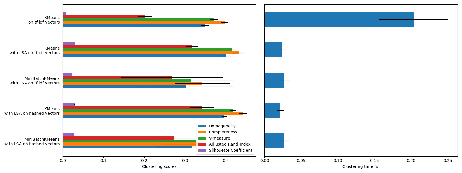
KMeans and MiniBatchKMeans
suffer from the phenomenon called the Curse of Dimensionality for high dimensional
datasets such as text data. That is the reason why the overall scores improve
when using LSA. Using LSA reduced data also improves the stability and
requires lower clustering time, though keep in mind that the LSA step itself
takes a long time, especially with hashed vectors.
The Silhouette Coefficient is defined between 0 and 1. In all cases we obtain values close to 0 (even if they improve a bit after using LSA) because its definition requires measuring distances, in contrast with other evaluation metrics such as the V-measure and the Adjusted Rand Index which are only based on cluster assignments rather than distances. Notice that strictly speaking, one should not compare the Silhouette Coefficient between spaces of different dimension, due to the different notions of distance they imply.
The homogeneity, completeness and hence v-measure metrics do not yield a baseline with regards to random labeling: this means that depending on the number of samples, clusters and ground truth classes, a completely random labeling will not always yield the same values. In particular random labeling won’t yield zero scores, especially when the number of clusters is large. This problem can safely be ignored when the number of samples is more than a thousand and the number of clusters is less than 10, which is the case of the present example. For smaller sample sizes or larger number of clusters it is safer to use an adjusted index such as the Adjusted Rand Index (ARI). See the example Adjustment for chance in clustering performance evaluation for a demo on the effect of random labeling.
The size of the error bars show that MiniBatchKMeans
is less stable than KMeans for this relatively small
dataset. It is more interesting to use when the number of samples is much
bigger, but it can come at the expense of a small degradation in clustering
quality compared to the traditional k-means algorithm.
Total running time of the script: (0 minutes 7.166 seconds)
Related examples
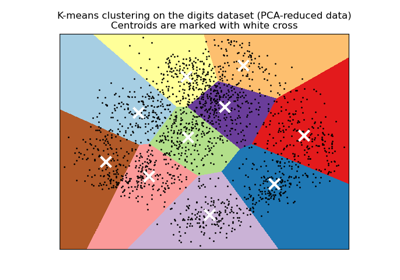
A demo of K-Means clustering on the handwritten digits data

Biclustering documents with the Spectral Co-clustering algorithm
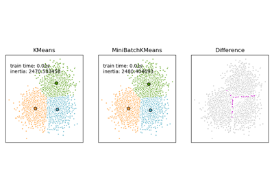
Comparison of the K-Means and MiniBatchKMeans clustering algorithms
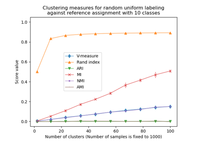
Adjustment for chance in clustering performance evaluation
Classification of text documents using sparse features