This is documentation for an old release of Scikit-learn (version 1.2). Try the latest stable release (version 1.6) or development (unstable) versions.

Putting it all together

Pipelining

We have seen that some estimators can transform data and that some estimators can predict variables. We can also create combined estimators:

from sklearn.decomposition import PCA
from sklearn.linear_model import LogisticRegression
from sklearn.pipeline import Pipeline
from sklearn.model_selection import GridSearchCV
from sklearn.preprocessing import StandardScaler

# Define a pipeline to search for the best combination of PCA truncation
# and classifier regularization.
pca = PCA()
# Define a Standard Scaler to normalize inputs
scaler = StandardScaler()

# set the tolerance to a large value to make the example faster
logistic = LogisticRegression(max_iter=10000, tol=0.1)
pipe = Pipeline(steps=[("scaler", scaler), ("pca", pca), ("logistic", logistic)])

X_digits, y_digits = datasets.load_digits(return_X_y=True)
# Parameters of pipelines can be set using '__' separated parameter names:
param_grid = {
    "pca__n_components": [5, 15, 30, 45, 60],
    "logistic__C": np.logspace(-4, 4, 4),
}
search = GridSearchCV(pipe, param_grid, n_jobs=2)
search.fit(X_digits, y_digits)
print("Best parameter (CV score=%0.3f):" % search.best_score_)
print(search.best_params_)

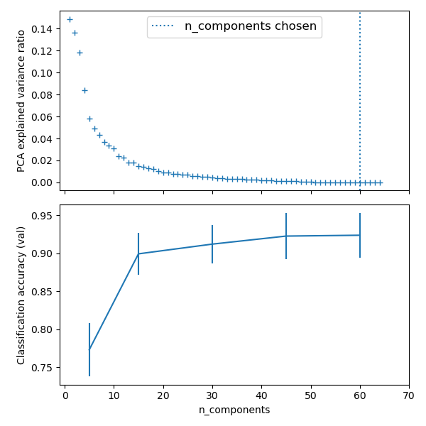
# Plot the PCA spectrum
pca.fit(X_digits)

fig, (ax0, ax1) = plt.subplots(nrows=2, sharex=True, figsize=(6, 6))
ax0.plot(
    np.arange(1, pca.n_components_ + 1), pca.explained_variance_ratio_, "+", linewidth=2
)
ax0.set_ylabel("PCA explained variance ratio")

ax0.axvline(
    search.best_estimator_.named_steps["pca"].n_components,
    linestyle=":",
    label="n_components chosen",
)

Face recognition with eigenfaces

The dataset used in this example is a preprocessed excerpt of the “Labeled Faces in the Wild”, also known as LFW:

http://vis-www.cs.umass.edu/lfw/lfw-funneled.tgz (233MB)

"""
===================================================
Faces recognition example using eigenfaces and SVMs
===================================================

The dataset used in this example is a preprocessed excerpt of the
"Labeled Faces in the Wild", aka LFW_:

  http://vis-www.cs.umass.edu/lfw/lfw-funneled.tgz (233MB)

.. _LFW: http://vis-www.cs.umass.edu/lfw/

"""
# %%
from time import time
import matplotlib.pyplot as plt

from sklearn.model_selection import train_test_split
from sklearn.model_selection import RandomizedSearchCV
from sklearn.datasets import fetch_lfw_people
from sklearn.metrics import classification_report
from sklearn.metrics import ConfusionMatrixDisplay
from sklearn.preprocessing import StandardScaler
from sklearn.decomposition import PCA
from sklearn.svm import SVC
from sklearn.utils.fixes import loguniform


# %%
# Download the data, if not already on disk and load it as numpy arrays

lfw_people = fetch_lfw_people(min_faces_per_person=70, resize=0.4)

# introspect the images arrays to find the shapes (for plotting)
n_samples, h, w = lfw_people.images.shape

# for machine learning we use the 2 data directly (as relative pixel
# positions info is ignored by this model)
X = lfw_people.data
n_features = X.shape[1]

# the label to predict is the id of the person
y = lfw_people.target
target_names = lfw_people.target_names
n_classes = target_names.shape[0]

print("Total dataset size:")
print("n_samples: %d" % n_samples)
print("n_features: %d" % n_features)
print("n_classes: %d" % n_classes)


# %%
# Split into a training set and a test and keep 25% of the data for testing.

X_train, X_test, y_train, y_test = train_test_split(
    X, y, test_size=0.25, random_state=42
)

scaler = StandardScaler()
X_train = scaler.fit_transform(X_train)
X_test = scaler.transform(X_test)

# %%
# Compute a PCA (eigenfaces) on the face dataset (treated as unlabeled
# dataset): unsupervised feature extraction / dimensionality reduction

n_components = 150

print(
    "Extracting the top %d eigenfaces from %d faces" % (n_components, X_train.shape[0])
)
t0 = time()
pca = PCA(n_components=n_components, svd_solver="randomized", whiten=True).fit(X_train)
print("done in %0.3fs" % (time() - t0))

eigenfaces = pca.components_.reshape((n_components, h, w))

print("Projecting the input data on the eigenfaces orthonormal basis")
t0 = time()
X_train_pca = pca.transform(X_train)
X_test_pca = pca.transform(X_test)
print("done in %0.3fs" % (time() - t0))


# %%
# Train a SVM classification model

print("Fitting the classifier to the training set")
t0 = time()
param_grid = {
    "C": loguniform(1e3, 1e5),
    "gamma": loguniform(1e-4, 1e-1),
}
clf = RandomizedSearchCV(
    SVC(kernel="rbf", class_weight="balanced"), param_grid, n_iter=10
)
clf = clf.fit(X_train_pca, y_train)
print("done in %0.3fs" % (time() - t0))
print("Best estimator found by grid search:")
print(clf.best_estimator_)


# %%
# Quantitative evaluation of the model quality on the test set

print("Predicting people's names on the test set")
t0 = time()
y_pred = clf.predict(X_test_pca)
print("done in %0.3fs" % (time() - t0))

print(classification_report(y_test, y_pred, target_names=target_names))
ConfusionMatrixDisplay.from_estimator(
    clf, X_test_pca, y_test, display_labels=target_names, xticks_rotation="vertical"
)
plt.tight_layout()
plt.show()


# %%
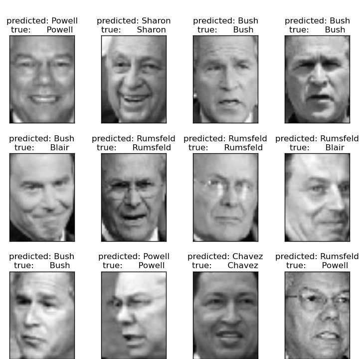
# Qualitative evaluation of the predictions using matplotlib


def plot_gallery(images, titles, h, w, n_row=3, n_col=4):
    """Helper function to plot a gallery of portraits"""
    plt.figure(figsize=(1.8 * n_col, 2.4 * n_row))
    plt.subplots_adjust(bottom=0, left=0.01, right=0.99, top=0.90, hspace=0.35)
    for i in range(n_row * n_col):
        plt.subplot(n_row, n_col, i + 1)
        plt.imshow(images[i].reshape((h, w)), cmap=plt.cm.gray)
        plt.title(titles[i], size=12)
        plt.xticks(())
        plt.yticks(())


# %%
# plot the result of the prediction on a portion of the test set


def title(y_pred, y_test, target_names, i):
    pred_name = target_names[y_pred[i]].rsplit(" ", 1)[-1]
    true_name = target_names[y_test[i]].rsplit(" ", 1)[-1]
    return "predicted: %s\ntrue:      %s" % (pred_name, true_name)


prediction_titles = [
    title(y_pred, y_test, target_names, i) for i in range(y_pred.shape[0])
]

plot_gallery(X_test, prediction_titles, h, w)
# %%
# plot the gallery of the most significative eigenfaces

eigenface_titles = ["eigenface %d" % i for i in range(eigenfaces.shape[0])]
plot_gallery(eigenfaces, eigenface_titles, h, w)

plt.show()

# %%
# Face recognition problem would be much more effectively solved by training
# convolutional neural networks but this family of models is outside of the scope of
# the scikit-learn library. Interested readers should instead try to use pytorch or
# tensorflow to implement such models.

Prediction

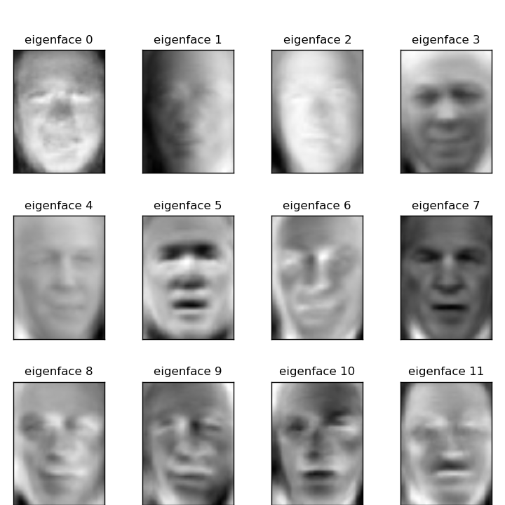
Eigenfaces

Expected results for the top 5 most represented people in the dataset:

                   precision    recall  f1-score   support

Gerhard_Schroeder       0.91      0.75      0.82        28
  Donald_Rumsfeld       0.84      0.82      0.83        33
       Tony_Blair       0.65      0.82      0.73        34
     Colin_Powell       0.78      0.88      0.83        58
    George_W_Bush       0.93      0.86      0.90       129

      avg / total       0.86      0.84      0.85       282

Open problem: Stock Market Structure

Can we predict the variation in stock prices for Google over a given time frame?

Learning a graph structure