sklearn.linear_model.SGDOneClassSVM

class sklearn.linear_model.SGDOneClassSVM(nu=0.5, fit_intercept=True, max_iter=1000, tol=0.001, shuffle=True, verbose=0, random_state=None, learning_rate='optimal', eta0=0.0, power_t=0.5, warm_start=False, average=False)

Solves linear One-Class SVM using Stochastic Gradient Descent.

This implementation is meant to be used with a kernel approximation technique (e.g. sklearn.kernel_approximation.Nystroem) to obtain results similar to sklearn.svm.OneClassSVM which uses a Gaussian kernel by default.

Read more in the User Guide.

New in version 1.0.

Parameters:

nufloat, default=0.5

The nu parameter of the One Class SVM: an upper bound on the fraction of training errors and a lower bound of the fraction of support vectors. Should be in the interval (0, 1]. By default 0.5 will be taken.

fit_interceptbool, default=True

Whether the intercept should be estimated or not. Defaults to True.

max_iterint, default=1000

The maximum number of passes over the training data (aka epochs). It only impacts the behavior in the fit method, and not the partial_fit. Defaults to 1000.

tolfloat or None, default=1e-3

The stopping criterion. If it is not None, the iterations will stop when (loss > previous_loss - tol). Defaults to 1e-3.

shufflebool, default=True

Whether or not the training data should be shuffled after each epoch. Defaults to True.

verboseint, default=0

The verbosity level.

random_stateint, RandomState instance or None, default=None

The seed of the pseudo random number generator to use when shuffling the data. If int, random_state is the seed used by the random number generator; If RandomState instance, random_state is the random number generator; If None, the random number generator is the RandomState instance used by np.random.

learning_rate{‘constant’, ‘optimal’, ‘invscaling’, ‘adaptive’}, default=’optimal’

The learning rate schedule to use with fit. (If using partial_fit, learning rate must be controlled directly).

• ‘constant’: eta = eta0

• ‘optimal’: eta = 1.0 / (alpha * (t + t0)) where t0 is chosen by a heuristic proposed by Leon Bottou.

• ‘invscaling’: eta = eta0 / pow(t, power_t)

• ‘adaptive’: eta = eta0, as long as the training keeps decreasing. Each time n_iter_no_change consecutive epochs fail to decrease the training loss by tol or fail to increase validation score by tol if early_stopping is True, the current learning rate is divided by 5.

eta0float, default=0.0

The initial learning rate for the ‘constant’, ‘invscaling’ or ‘adaptive’ schedules. The default value is 0.0 as eta0 is not used by the default schedule ‘optimal’.

power_tfloat, default=0.5

The exponent for inverse scaling learning rate [default 0.5].

warm_startbool, default=False

When set to True, reuse the solution of the previous call to fit as initialization, otherwise, just erase the previous solution. See the Glossary.

Repeatedly calling fit or partial_fit when warm_start is True can result in a different solution than when calling fit a single time because of the way the data is shuffled. If a dynamic learning rate is used, the learning rate is adapted depending on the number of samples already seen. Calling fit resets this counter, while partial_fit will result in increasing the existing counter.

averagebool or int, default=False

When set to True, computes the averaged SGD weights and stores the result in the coef_ attribute. If set to an int greater than 1, averaging will begin once the total number of samples seen reaches average. So average=10 will begin averaging after seeing 10 samples.

Attributes:

coef_ndarray of shape (1, n_features)

Weights assigned to the features.

offset_ndarray of shape (1,)

Offset used to define the decision function from the raw scores. We have the relation: decision_function = score_samples - offset.

n_iter_int

The actual number of iterations to reach the stopping criterion.

t_int

Number of weight updates performed during training. Same as (n_iter_ * n_samples + 1).

loss_function_concrete LossFunction

n_features_in_int

Number of features seen during fit.

New in version 0.24.

feature_names_in_ndarray of shape (n_features_in_,)

Names of features seen during fit. Defined only when X has feature names that are all strings.

New in version 1.0.

See also

sklearn.svm.OneClassSVM

Unsupervised Outlier Detection.

Notes

This estimator has a linear complexity in the number of training samples and is thus better suited than the sklearn.svm.OneClassSVM implementation for datasets with a large number of training samples (say > 10,000).

Examples

>>> import numpy as np
>>> from sklearn import linear_model
>>> X = np.array([[-1, -1], [-2, -1], [1, 1], [2, 1]])
>>> clf = linear_model.SGDOneClassSVM(random_state=42)
>>> clf.fit(X)
SGDOneClassSVM(random_state=42)

>>> print(clf.predict([[4, 4]]))
[1]

Methods

decision_function(X)	Signed distance to the separating hyperplane.
densify()	Convert coefficient matrix to dense array format.
fit(X[, y, coef_init, offset_init, ...])	Fit linear One-Class SVM with Stochastic Gradient Descent.
fit_predict(X[, y])	Perform fit on X and returns labels for X.
get_params([deep])	Get parameters for this estimator.
partial_fit(X[, y, sample_weight])	Fit linear One-Class SVM with Stochastic Gradient Descent.
predict(X)	Return labels (1 inlier, -1 outlier) of the samples.
score_samples(X)	Raw scoring function of the samples.
set_params(**params)	Set the parameters of this estimator.
sparsify()	Convert coefficient matrix to sparse format.

decision_function(X)

Signed distance to the separating hyperplane.

Signed distance is positive for an inlier and negative for an outlier.

Parameters:

X{array-like, sparse matrix}, shape (n_samples, n_features)

Testing data.

Returns:

decarray-like, shape (n_samples,)

Decision function values of the samples.

densify()

Convert coefficient matrix to dense array format.

Converts the coef_ member (back) to a numpy.ndarray. This is the default format of coef_ and is required for fitting, so calling this method is only required on models that have previously been sparsified; otherwise, it is a no-op.

Returns:

self

Fitted estimator.

fit(X, y=None, coef_init=None, offset_init=None, sample_weight=None)

Fit linear One-Class SVM with Stochastic Gradient Descent.

This solves an equivalent optimization problem of the One-Class SVM primal optimization problem and returns a weight vector w and an offset rho such that the decision function is given by <w, x> - rho.

Parameters:

X{array-like, sparse matrix}, shape (n_samples, n_features)

Training data.

yIgnored

Not used, present for API consistency by convention.

coef_initarray, shape (n_classes, n_features)

The initial coefficients to warm-start the optimization.

offset_initarray, shape (n_classes,)

The initial offset to warm-start the optimization.

sample_weightarray-like, shape (n_samples,), optional

Weights applied to individual samples. If not provided, uniform weights are assumed. These weights will be multiplied with class_weight (passed through the constructor) if class_weight is specified.

Returns:

selfobject

Returns a fitted instance of self.

fit_predict(X, y=None)

Perform fit on X and returns labels for X.

Returns -1 for outliers and 1 for inliers.

Parameters:

X{array-like, sparse matrix} of shape (n_samples, n_features)

The input samples.

yIgnored

Not used, present for API consistency by convention.

Returns:

yndarray of shape (n_samples,)

1 for inliers, -1 for outliers.

get_params(deep=True)

Get parameters for this estimator.

Parameters:

deepbool, default=True

If True, will return the parameters for this estimator and contained subobjects that are estimators.

Returns:

paramsdict

Parameter names mapped to their values.

partial_fit(X, y=None, sample_weight=None)

Fit linear One-Class SVM with Stochastic Gradient Descent.

Parameters:

X{array-like, sparse matrix}, shape (n_samples, n_features)

Subset of the training data.

yIgnored

Not used, present for API consistency by convention.

sample_weightarray-like, shape (n_samples,), optional

Weights applied to individual samples. If not provided, uniform weights are assumed.

Returns:

selfobject

Returns a fitted instance of self.

predict(X)

Return labels (1 inlier, -1 outlier) of the samples.

Parameters:

X{array-like, sparse matrix}, shape (n_samples, n_features)

Testing data.

Returns:

yarray, shape (n_samples,)

Labels of the samples.

score_samples(X)

Raw scoring function of the samples.

Parameters:

X{array-like, sparse matrix}, shape (n_samples, n_features)

Testing data.

Returns:

score_samplesarray-like, shape (n_samples,)

Unshiffted scoring function values of the samples.

set_params(**params)

Set the parameters of this estimator.

The method works on simple estimators as well as on nested objects (such as Pipeline). The latter have parameters of the form <component>__<parameter> so that it’s possible to update each component of a nested object.

Parameters:

**paramsdict

Estimator parameters.

Returns:

selfestimator instance

Estimator instance.

sparsify()

Convert coefficient matrix to sparse format.

Converts the coef_ member to a scipy.sparse matrix, which for L1-regularized models can be much more memory- and storage-efficient than the usual numpy.ndarray representation.

The intercept_ member is not converted.

Returns:

self

Fitted estimator.

Notes

For non-sparse models, i.e. when there are not many zeros in coef_, this may actually increase memory usage, so use this method with care. A rule of thumb is that the number of zero elements, which can be computed with (coef_ == 0).sum(), must be more than 50% for this to provide significant benefits.

After calling this method, further fitting with the partial_fit method (if any) will not work until you call densify.

Examples using sklearn.linear_model.SGDOneClassSVM

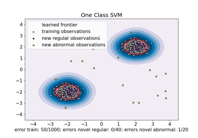
One-Class SVM versus One-Class SVM using Stochastic Gradient Descent

One-Class SVM versus One-Class SVM using Stochastic Gradient Descent

Comparing anomaly detection algorithms for outlier detection on toy datasets

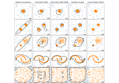
Comparing anomaly detection algorithms for outlier detection on toy datasets