Scaling the regularization parameter for SVCs

The following example illustrates the effect of scaling the regularization parameter when using Support Vector Machines for classification. For SVC classification, we are interested in a risk minimization for the equation:

\[C \sum_{i=1, n} \mathcal{L} (f(x_i), y_i) + \Omega (w)\]

where

• \(C\) is used to set the amount of regularization

• \(\mathcal{L}\) is a loss function of our samples and our model parameters.

• \(\Omega\) is a penalty function of our model parameters

If we consider the loss function to be the individual error per sample, then the data-fit term, or the sum of the error for each sample, will increase as we add more samples. The penalization term, however, will not increase.

When using, for example, cross validation, to set the amount of regularization with C, there will be a different amount of samples between the main problem and the smaller problems within the folds of the cross validation.

Since our loss function is dependent on the amount of samples, the latter will influence the selected value of C. The question that arises is “How do we optimally adjust C to account for the different amount of training samples?”

In the remainder of this example, we will investigate the effect of scaling the value of the regularization parameter C in regards to the number of samples for both L1 and L2 penalty. We will generate some synthetic datasets that are appropriate for each type of regularization.

# Author: Andreas Mueller <amueller@ais.uni-bonn.de>
#         Jaques Grobler <jaques.grobler@inria.fr>
# License: BSD 3 clause

L1-penalty case

In the L1 case, theory says that prediction consistency (i.e. that under given hypothesis, the estimator learned predicts as well as a model knowing the true distribution) is not possible because of the bias of the L1. It does say, however, that model consistency, in terms of finding the right set of non-zero parameters as well as their signs, can be achieved by scaling C.

We will demonstrate this effect by using a synthetic dataset. This dataset will be sparse, meaning that only a few features will be informative and useful for the model.

from sklearn.datasets import make_classification

n_samples, n_features = 100, 300
X, y = make_classification(
    n_samples=n_samples, n_features=n_features, n_informative=5, random_state=1
)

Now, we can define a linear SVC with the l1 penalty.

from sklearn.svm import LinearSVC

model_l1 = LinearSVC(penalty="l1", loss="squared_hinge", dual=False, tol=1e-3)

We will compute the mean test score for different values of C.

import numpy as np
import pandas as pd
from sklearn.model_selection import validation_curve, ShuffleSplit

Cs = np.logspace(-2.3, -1.3, 10)
train_sizes = np.linspace(0.3, 0.7, 3)
labels = [f"fraction: {train_size}" for train_size in train_sizes]

results = {"C": Cs}
for label, train_size in zip(labels, train_sizes):
    cv = ShuffleSplit(train_size=train_size, test_size=0.3, n_splits=50, random_state=1)
    train_scores, test_scores = validation_curve(
        model_l1, X, y, param_name="C", param_range=Cs, cv=cv
    )
    results[label] = test_scores.mean(axis=1)
results = pd.DataFrame(results)

import matplotlib.pyplot as plt

fig, axes = plt.subplots(nrows=1, ncols=2, sharey=True, figsize=(12, 6))

# plot results without scaling C
results.plot(x="C", ax=axes[0], logx=True)
axes[0].set_ylabel("CV score")
axes[0].set_title("No scaling")

# plot results by scaling C
for train_size_idx, label in enumerate(labels):
    results_scaled = results[[label]].assign(
        C_scaled=Cs * float(n_samples * train_sizes[train_size_idx])
    )
    results_scaled.plot(x="C_scaled", ax=axes[1], logx=True, label=label)
axes[1].set_title("Scaling C by 1 / n_samples")

_ = fig.suptitle("Effect of scaling C with L1 penalty")

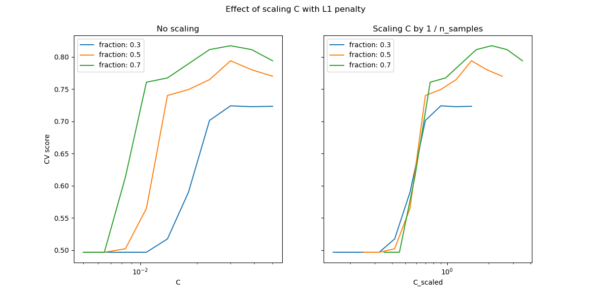
Here, we observe that the cross-validation-error correlates best with the test-error, when scaling our C with the number of samples, n.

L2-penalty case

We can repeat a similar experiment with the l2 penalty. In this case, we don’t need to use a sparse dataset.

In this case, the theory says that in order to achieve prediction consistency, the penalty parameter should be kept constant as the number of samples grow.

So we will repeat the same experiment by creating a linear SVC classifier with the l2 penalty and check the test score via cross-validation and plot the results with and without scaling the parameter C.

rng = np.random.RandomState(1)
y = np.sign(0.5 - rng.rand(n_samples))
X = rng.randn(n_samples, n_features // 5) + y[:, np.newaxis]
X += 5 * rng.randn(n_samples, n_features // 5)

model_l2 = LinearSVC(penalty="l2", loss="squared_hinge", dual=True)
Cs = np.logspace(-4.5, -2, 10)

labels = [f"fraction: {train_size}" for train_size in train_sizes]
results = {"C": Cs}
for label, train_size in zip(labels, train_sizes):
    cv = ShuffleSplit(train_size=train_size, test_size=0.3, n_splits=50, random_state=1)
    train_scores, test_scores = validation_curve(
        model_l2, X, y, param_name="C", param_range=Cs, cv=cv
    )
    results[label] = test_scores.mean(axis=1)
results = pd.DataFrame(results)

import matplotlib.pyplot as plt

fig, axes = plt.subplots(nrows=1, ncols=2, sharey=True, figsize=(12, 6))

# plot results without scaling C
results.plot(x="C", ax=axes[0], logx=True)
axes[0].set_ylabel("CV score")
axes[0].set_title("No scaling")

# plot results by scaling C
for train_size_idx, label in enumerate(labels):
    results_scaled = results[[label]].assign(
        C_scaled=Cs * float(n_samples * train_sizes[train_size_idx])
    )
    results_scaled.plot(x="C_scaled", ax=axes[1], logx=True, label=label)
axes[1].set_title("Scaling C by 1 / n_samples")

_ = fig.suptitle("Effect of scaling C with L2 penalty")

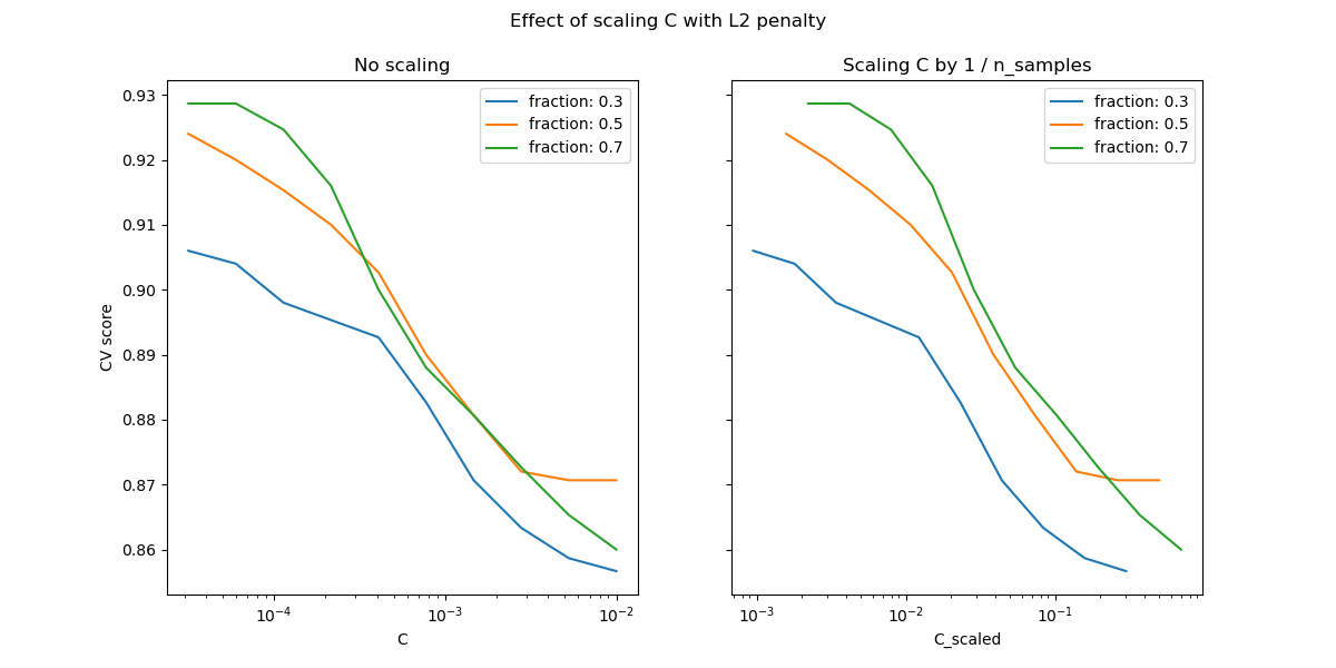
So or the L2 penalty case, the best result comes from the case where C is not scaled.

plt.show()