Note
Click here to download the full example code or to run this example in your browser via Binder
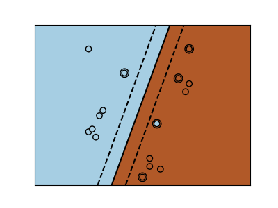
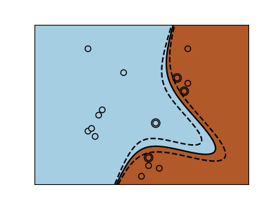
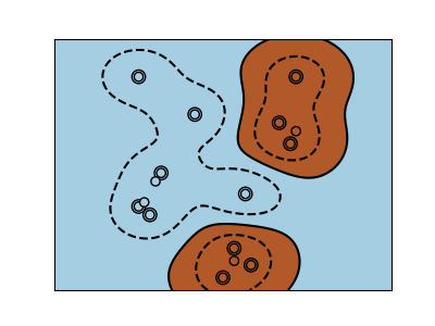
SVM-Kernels
Three different types of SVM-Kernels are displayed below. The polynomial and RBF are especially useful when the data-points are not linearly separable.
# Code source: Gaël Varoquaux
# License: BSD 3 clause

import numpy as np
import matplotlib.pyplot as plt
from sklearn import svm


# Our dataset and targets
X = np.c_[
    (0.4, -0.7),
    (-1.5, -1),
    (-1.4, -0.9),
    (-1.3, -1.2),
    (-1.1, -0.2),
    (-1.2, -0.4),
    (-0.5, 1.2),
    (-1.5, 2.1),
    (1, 1),
    # --
    (1.3, 0.8),
    (1.2, 0.5),
    (0.2, -2),
    (0.5, -2.4),
    (0.2, -2.3),
    (0, -2.7),
    (1.3, 2.1),
].T
Y = [0] * 8 + [1] * 8

# figure number
fignum = 1

# fit the model
for kernel in ("linear", "poly", "rbf"):
    clf = svm.SVC(kernel=kernel, gamma=2)
    clf.fit(X, Y)

    # plot the line, the points, and the nearest vectors to the plane
    plt.figure(fignum, figsize=(4, 3))
    plt.clf()

    plt.scatter(
        clf.support_vectors_[:, 0],
        clf.support_vectors_[:, 1],
        s=80,
        facecolors="none",
        zorder=10,
        edgecolors="k",
    )
    plt.scatter(X[:, 0], X[:, 1], c=Y, zorder=10, cmap=plt.cm.Paired, edgecolors="k")

    plt.axis("tight")
    x_min = -3
    x_max = 3
    y_min = -3
    y_max = 3

    XX, YY = np.mgrid[x_min:x_max:200j, y_min:y_max:200j]
    Z = clf.decision_function(np.c_[XX.ravel(), YY.ravel()])

    # Put the result into a color plot
    Z = Z.reshape(XX.shape)
    plt.figure(fignum, figsize=(4, 3))
    plt.pcolormesh(XX, YY, Z > 0, cmap=plt.cm.Paired)
    plt.contour(
        XX,
        YY,
        Z,
        colors=["k", "k", "k"],
        linestyles=["--", "-", "--"],
        levels=[-0.5, 0, 0.5],
    )

    plt.xlim(x_min, x_max)
    plt.ylim(y_min, y_max)

    plt.xticks(())
    plt.yticks(())
    fignum = fignum + 1
plt.show()
Total running time of the script: ( 0 minutes 0.196 seconds)