Receiver Operating Characteristic (ROC) with cross validation

This example presents how to estimate and visualize the variance of the Receiver Operating Characteristic (ROC) metric using cross-validation.

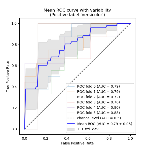
ROC curves typically feature true positive rate (TPR) on the Y axis, and false positive rate (FPR) on the X axis. This means that the top left corner of the plot is the “ideal” point - a FPR of zero, and a TPR of one. This is not very realistic, but it does mean that a larger Area Under the Curve (AUC) is usually better. The “steepness” of ROC curves is also important, since it is ideal to maximize the TPR while minimizing the FPR.

This example shows the ROC response of different datasets, created from K-fold cross-validation. Taking all of these curves, it is possible to calculate the mean AUC, and see the variance of the curve when the training set is split into different subsets. This roughly shows how the classifier output is affected by changes in the training data, and how different the splits generated by K-fold cross-validation are from one another.

Note

See Multiclass Receiver Operating Characteristic (ROC) for a complement of the present example explaining the averaging strategies to generalize the metrics for multiclass classifiers.

Load and prepare data

We import the Iris plants dataset which contains 3 classes, each one corresponding to a type of iris plant. One class is linearly separable from the other 2; the latter are not linearly separable from each other.

In the following we binarize the dataset by dropping the “virginica” class (class_id=2). This means that the “versicolor” class (class_id=1) is regarded as the positive class and “setosa” as the negative class (class_id=0).

import numpy as np
from sklearn.datasets import load_iris

iris = load_iris()
target_names = iris.target_names
X, y = iris.data, iris.target
X, y = X[y != 2], y[y != 2]
n_samples, n_features = X.shape

We also add noisy features to make the problem harder.

random_state = np.random.RandomState(0)
X = np.concatenate([X, random_state.randn(n_samples, 200 * n_features)], axis=1)

Classification and ROC analysis

Here we run a SVC classifier with cross-validation and plot the ROC curves fold-wise. Notice that the baseline to define the chance level (dashed ROC curve) is a classifier that would always predict the most frequent class.

import matplotlib.pyplot as plt

from sklearn import svm
from sklearn.metrics import auc
from sklearn.metrics import RocCurveDisplay
from sklearn.model_selection import StratifiedKFold

cv = StratifiedKFold(n_splits=6)
classifier = svm.SVC(kernel="linear", probability=True, random_state=random_state)

tprs = []
aucs = []
mean_fpr = np.linspace(0, 1, 100)

fig, ax = plt.subplots(figsize=(6, 6))
for fold, (train, test) in enumerate(cv.split(X, y)):
    classifier.fit(X[train], y[train])
    viz = RocCurveDisplay.from_estimator(
        classifier,
        X[test],
        y[test],
        name=f"ROC fold {fold}",
        alpha=0.3,
        lw=1,
        ax=ax,
    )
    interp_tpr = np.interp(mean_fpr, viz.fpr, viz.tpr)
    interp_tpr[0] = 0.0
    tprs.append(interp_tpr)
    aucs.append(viz.roc_auc)
ax.plot([0, 1], [0, 1], "k--", label="chance level (AUC = 0.5)")

mean_tpr = np.mean(tprs, axis=0)
mean_tpr[-1] = 1.0
mean_auc = auc(mean_fpr, mean_tpr)
std_auc = np.std(aucs)
ax.plot(
    mean_fpr,
    mean_tpr,
    color="b",
    label=r"Mean ROC (AUC = %0.2f $\pm$ %0.2f)" % (mean_auc, std_auc),
    lw=2,
    alpha=0.8,
)

std_tpr = np.std(tprs, axis=0)
tprs_upper = np.minimum(mean_tpr + std_tpr, 1)
tprs_lower = np.maximum(mean_tpr - std_tpr, 0)
ax.fill_between(
    mean_fpr,
    tprs_lower,
    tprs_upper,
    color="grey",
    alpha=0.2,
    label=r"$\pm$ 1 std. dev.",
)

ax.set(
    xlim=[-0.05, 1.05],
    ylim=[-0.05, 1.05],
    xlabel="False Positive Rate",
    ylabel="True Positive Rate",
    title=f"Mean ROC curve with variability\n(Positive label '{target_names[1]}')",
)
ax.axis("square")
ax.legend(loc="lower right")
plt.show()