This is documentation for an old release of Scikit-learn (version 1.2). Try the latest stable release (version 1.6) or development (unstable) versions.

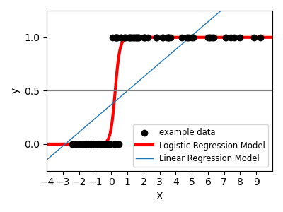
Logistic function

Shown in the plot is how the logistic regression would, in this synthetic dataset, classify values as either 0 or 1, i.e. class one or two, using the logistic curve.

# Code source: Gael Varoquaux
# License: BSD 3 clause

import matplotlib.pyplot as plt
import numpy as np
from scipy.special import expit
from sklearn.linear_model import LinearRegression, LogisticRegression

# Generate a toy dataset, it's just a straight line with some Gaussian noise:
xmin, xmax = -5, 5
n_samples = 100
np.random.seed(0)
X = np.random.normal(size=n_samples)
y = (X > 0).astype(float)
X[X > 0] *= 4
X += 0.3 * np.random.normal(size=n_samples)

X = X[:, np.newaxis]

# Fit the classifier
clf = LogisticRegression(C=1e5)
clf.fit(X, y)

# and plot the result
plt.figure(1, figsize=(4, 3))
plt.clf()
plt.scatter(X.ravel(), y, label="example data", color="black", zorder=20)
X_test = np.linspace(-5, 10, 300)

loss = expit(X_test * clf.coef_ + clf.intercept_).ravel()
plt.plot(X_test, loss, label="Logistic Regression Model", color="red", linewidth=3)

ols = LinearRegression()
ols.fit(X, y)
plt.plot(
    X_test,
    ols.coef_ * X_test + ols.intercept_,
    label="Linear Regression Model",
    linewidth=1,
)
plt.axhline(0.5, color=".5")

plt.ylabel("y")
plt.xlabel("X")
plt.xticks(range(-5, 10))
plt.yticks([0, 0.5, 1])
plt.ylim(-0.25, 1.25)
plt.xlim(-4, 10)
plt.legend(
    loc="lower right",
    fontsize="small",
)
plt.tight_layout()
plt.show()