Monotonic Constraints

This example illustrates the effect of monotonic constraints on a gradient boosting estimator.

We build an artificial dataset where the target value is in general positively correlated with the first feature (with some random and non-random variations), and in general negatively correlated with the second feature.

By imposing a monotonic increase or a monotonic decrease constraint, respectively, on the features during the learning process, the estimator is able to properly follow the general trend instead of being subject to the variations.

This example was inspired by the XGBoost documentation.

from sklearn.ensemble import HistGradientBoostingRegressor
from sklearn.inspection import PartialDependenceDisplay
import numpy as np
import matplotlib.pyplot as plt


rng = np.random.RandomState(0)

n_samples = 1000
f_0 = rng.rand(n_samples)
f_1 = rng.rand(n_samples)
X = np.c_[f_0, f_1]
noise = rng.normal(loc=0.0, scale=0.01, size=n_samples)

# y is positively correlated with f_0, and negatively correlated with f_1
y = 5 * f_0 + np.sin(10 * np.pi * f_0) - 5 * f_1 - np.cos(10 * np.pi * f_1) + noise

Fit a first model on this dataset without any constraints.

gbdt_no_cst = HistGradientBoostingRegressor()
gbdt_no_cst.fit(X, y)

HistGradientBoostingRegressor()

In a Jupyter environment, please rerun this cell to show the HTML representation or trust the notebook.
On GitHub, the HTML representation is unable to render, please try loading this page with nbviewer.org.

Fit a second model on this dataset with monotonic increase (1) and a monotonic decrease (-1) constraints, respectively.

gbdt_with_monotonic_cst = HistGradientBoostingRegressor(monotonic_cst=[1, -1])
gbdt_with_monotonic_cst.fit(X, y)

HistGradientBoostingRegressor(monotonic_cst=[1, -1])

In a Jupyter environment, please rerun this cell to show the HTML representation or trust the notebook.
On GitHub, the HTML representation is unable to render, please try loading this page with nbviewer.org.

Let’s display the partial dependence of the predictions on the two features.

fig, ax = plt.subplots()
disp = PartialDependenceDisplay.from_estimator(
    gbdt_no_cst,
    X,
    features=[0, 1],
    feature_names=(
        "First feature",
        "Second feature",
    ),
    line_kw={"linewidth": 4, "label": "unconstrained", "color": "tab:blue"},
    ax=ax,
)
PartialDependenceDisplay.from_estimator(
    gbdt_with_monotonic_cst,
    X,
    features=[0, 1],
    line_kw={"linewidth": 4, "label": "constrained", "color": "tab:orange"},
    ax=disp.axes_,
)

for f_idx in (0, 1):
    disp.axes_[0, f_idx].plot(
        X[:, f_idx], y, "o", alpha=0.3, zorder=-1, color="tab:green"
    )
    disp.axes_[0, f_idx].set_ylim(-6, 6)

plt.legend()
fig.suptitle("Monotonic constraints effect on partial dependences")
plt.show()

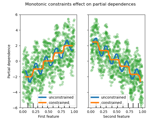
We can see that the predictions of the unconstrained model capture the oscillations of the data while the constrained model follows the general trend and ignores the local variations.

Using feature names to specify monotonic constraints

Note that if the training data has feature names, it’s possible to specifiy the monotonic constraints by passing a dictionary:

import pandas as pd

X_df = pd.DataFrame(X, columns=["f_0", "f_1"])

gbdt_with_monotonic_cst_df = HistGradientBoostingRegressor(
    monotonic_cst={"f_0": 1, "f_1": -1}
).fit(X_df, y)

np.allclose(
    gbdt_with_monotonic_cst_df.predict(X_df), gbdt_with_monotonic_cst.predict(X)
)

True