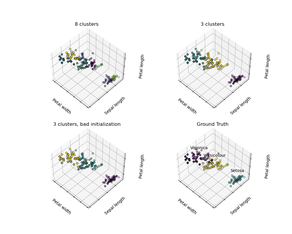
K-means Clustering

The plot shows:

• top left: What a K-means algorithm would yield using 8 clusters.

• top right: What the effect of a bad initialization is on the classification process: By setting n_init to only 1 (default is 10), the amount of times that the algorithm will be run with different centroid seeds is reduced.

• bottom left: What using eight clusters would deliver.

• bottom right: The ground truth.

# Code source: Gaël Varoquaux
# Modified for documentation by Jaques Grobler
# License: BSD 3 clause

import numpy as np
import matplotlib.pyplot as plt

# Though the following import is not directly being used, it is required
# for 3D projection to work with matplotlib < 3.2
import mpl_toolkits.mplot3d  # noqa: F401

from sklearn.cluster import KMeans
from sklearn import datasets

np.random.seed(5)

iris = datasets.load_iris()
X = iris.data
y = iris.target

estimators = [
    ("k_means_iris_8", KMeans(n_clusters=8, n_init="auto")),
    ("k_means_iris_3", KMeans(n_clusters=3, n_init="auto")),
    ("k_means_iris_bad_init", KMeans(n_clusters=3, n_init=1, init="random")),
]

fig = plt.figure(figsize=(10, 8))
titles = ["8 clusters", "3 clusters", "3 clusters, bad initialization"]
for idx, ((name, est), title) in enumerate(zip(estimators, titles)):
    ax = fig.add_subplot(2, 2, idx + 1, projection="3d", elev=48, azim=134)
    est.fit(X)
    labels = est.labels_

    ax.scatter(X[:, 3], X[:, 0], X[:, 2], c=labels.astype(float), edgecolor="k")

    ax.xaxis.set_ticklabels([])
    ax.yaxis.set_ticklabels([])
    ax.zaxis.set_ticklabels([])
    ax.set_xlabel("Petal width")
    ax.set_ylabel("Sepal length")
    ax.set_zlabel("Petal length")
    ax.set_title(title)

# Plot the ground truth
ax = fig.add_subplot(2, 2, 4, projection="3d", elev=48, azim=134)

for name, label in [("Setosa", 0), ("Versicolour", 1), ("Virginica", 2)]:
    ax.text3D(
        X[y == label, 3].mean(),
        X[y == label, 0].mean(),
        X[y == label, 2].mean() + 2,
        name,
        horizontalalignment="center",
        bbox=dict(alpha=0.2, edgecolor="w", facecolor="w"),
    )
# Reorder the labels to have colors matching the cluster results
y = np.choose(y, [1, 2, 0]).astype(float)
ax.scatter(X[:, 3], X[:, 0], X[:, 2], c=y, edgecolor="k")

ax.xaxis.set_ticklabels([])
ax.yaxis.set_ticklabels([])
ax.zaxis.set_ticklabels([])
ax.set_xlabel("Petal width")
ax.set_ylabel("Sepal length")
ax.set_zlabel("Petal length")
ax.set_title("Ground Truth")

plt.subplots_adjust(wspace=0.25, hspace=0.25)
plt.show()