Unsupervised learning: seeking representations of the data

Clustering: grouping observations together

The problem solved in clustering

Given the iris dataset, if we knew that there were 3 types of iris, but did not have access to a taxonomist to label them: we could try a clustering task: split the observations into well-separated group called clusters.

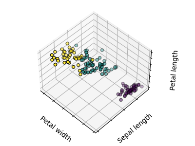
K-means clustering

Note that there exist a lot of different clustering criteria and associated algorithms. The simplest clustering algorithm is K-means.

>>> from sklearn import cluster, datasets
>>> X_iris, y_iris = datasets.load_iris(return_X_y=True)

>>> k_means = cluster.KMeans(n_clusters=3)
>>> k_means.fit(X_iris)
KMeans(n_clusters=3)
>>> print(k_means.labels_[::10])
[1 1 1 1 1 0 0 0 0 0 2 2 2 2 2]
>>> print(y_iris[::10])
[0 0 0 0 0 1 1 1 1 1 2 2 2 2 2]

Warning

There is absolutely no guarantee of recovering a ground truth. First, choosing the right number of clusters is hard. Second, the algorithm is sensitive to initialization, and can fall into local minima, although scikit-learn employs several tricks to mitigate this issue.

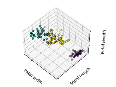
Bad initialization

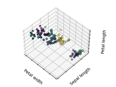
8 clusters

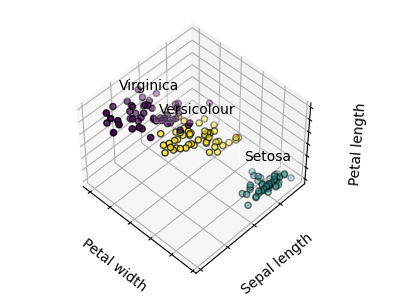
Ground truth

Don’t over-interpret clustering results

Application example: vector quantization

Clustering in general and KMeans, in particular, can be seen as a way of choosing a small number of exemplars to compress the information. The problem is sometimes known as vector quantization. For instance, this can be used to posterize an image:

>>> import scipy as sp
>>> try:
...    face = sp.face(gray=True)
... except AttributeError:
...    from scipy import misc
...    face = misc.face(gray=True)
>>> X = face.reshape((-1, 1)) # We need an (n_sample, n_feature) array
>>> k_means = cluster.KMeans(n_clusters=5, n_init=1)
>>> k_means.fit(X)
KMeans(n_clusters=5, n_init=1)
>>> values = k_means.cluster_centers_.squeeze()
>>> labels = k_means.labels_
>>> face_compressed = np.choose(labels, values)
>>> face_compressed.shape = face.shape

Raw image

K-means quantization

Equal bins

Image histogram

Hierarchical agglomerative clustering: Ward

A Hierarchical clustering method is a type of cluster analysis that aims to build a hierarchy of clusters. In general, the various approaches of this technique are either:

• Agglomerative - bottom-up approaches: each observation starts in its own cluster, and clusters are iteratively merged in such a way to minimize a linkage criterion. This approach is particularly interesting when the clusters of interest are made of only a few observations. When the number of clusters is large, it is much more computationally efficient than k-means.

• Divisive - top-down approaches: all observations start in one cluster, which is iteratively split as one moves down the hierarchy. For estimating large numbers of clusters, this approach is both slow (due to all observations starting as one cluster, which it splits recursively) and statistically ill-posed.

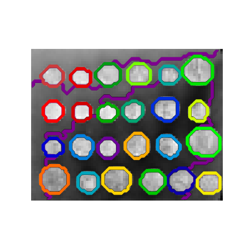
Connectivity-constrained clustering

With agglomerative clustering, it is possible to specify which samples can be clustered together by giving a connectivity graph. Graphs in scikit-learn are represented by their adjacency matrix. Often, a sparse matrix is used. This can be useful, for instance, to retrieve connected regions (sometimes also referred to as connected components) when clustering an image.

>>> from skimage.data import coins
>>> from scipy.ndimage import gaussian_filter
>>> from skimage.transform import rescale
>>> rescaled_coins = rescale(
...     gaussian_filter(coins(), sigma=2),
...     0.2, mode='reflect', anti_aliasing=False, multichannel=False
... )
>>> X = np.reshape(rescaled_coins, (-1, 1))

We need a vectorized version of the image. 'rescaled_coins' is a down-scaled version of the coins image to speed up the process:

>>> from sklearn.feature_extraction import grid_to_graph
>>> connectivity = grid_to_graph(*rescaled_coins.shape)

Define the graph structure of the data. Pixels connected to their neighbors:

>>> n_clusters = 27  # number of regions

>>> from sklearn.cluster import AgglomerativeClustering
>>> ward = AgglomerativeClustering(n_clusters=n_clusters, linkage='ward',
...                                connectivity=connectivity)
>>> ward.fit(X)
AgglomerativeClustering(connectivity=..., n_clusters=27)
>>> label = np.reshape(ward.labels_, rescaled_coins.shape)

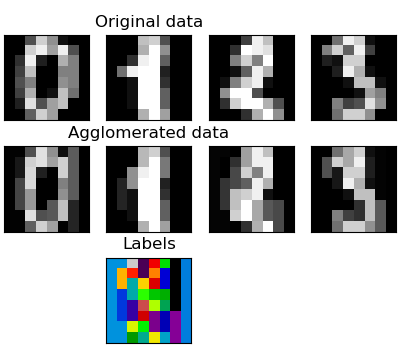
Feature agglomeration

We have seen that sparsity could be used to mitigate the curse of dimensionality, i.e an insufficient amount of observations compared to the number of features. Another approach is to merge together similar features: feature agglomeration. This approach can be implemented by clustering in the feature direction, in other words clustering the transposed data.

>>> digits = datasets.load_digits()
>>> images = digits.images
>>> X = np.reshape(images, (len(images), -1))
>>> connectivity = grid_to_graph(*images[0].shape)

>>> agglo = cluster.FeatureAgglomeration(connectivity=connectivity,
...                                      n_clusters=32)
>>> agglo.fit(X)
FeatureAgglomeration(connectivity=..., n_clusters=32)
>>> X_reduced = agglo.transform(X)

>>> X_approx = agglo.inverse_transform(X_reduced)
>>> images_approx = np.reshape(X_approx, images.shape)

transform and inverse_transform methods

Some estimators expose a transform method, for instance to reduce the dimensionality of the dataset.

Decompositions: from a signal to components and loadings

Components and loadings

If X is our multivariate data, then the problem that we are trying to solve is to rewrite it on a different observational basis: we want to learn loadings L and a set of components C such that X = L C. Different criteria exist to choose the components

Principal component analysis: PCA

Principal component analysis (PCA) selects the successive components that explain the maximum variance in the signal.

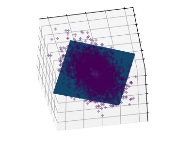
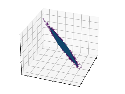
The point cloud spanned by the observations above is very flat in one direction: one of the three univariate features can almost be exactly computed using the other two. PCA finds the directions in which the data is not flat

When used to transform data, PCA can reduce the dimensionality of the data by projecting on a principal subspace.

>>> # Create a signal with only 2 useful dimensions
>>> x1 = np.random.normal(size=100)
>>> x2 = np.random.normal(size=100)
>>> x3 = x1 + x2
>>> X = np.c_[x1, x2, x3]

>>> from sklearn import decomposition
>>> pca = decomposition.PCA()
>>> pca.fit(X)
PCA()
>>> print(pca.explained_variance_)  
[  2.18565811e+00   1.19346747e+00   8.43026679e-32]

>>> # As we can see, only the 2 first components are useful
>>> pca.n_components = 2
>>> X_reduced = pca.fit_transform(X)
>>> X_reduced.shape
(100, 2)

Independent Component Analysis: ICA

Independent component analysis (ICA) selects components so that the distribution of their loadings carries a maximum amount of independent information. It is able to recover non-Gaussian independent signals:

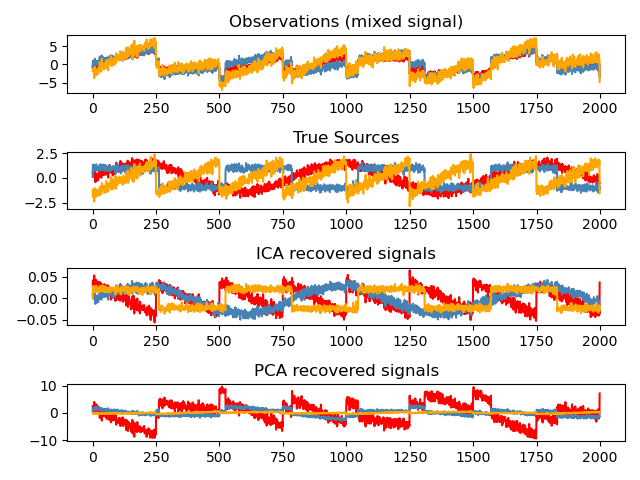
>>> # Generate sample data
>>> import numpy as np
>>> from scipy import signal
>>> time = np.linspace(0, 10, 2000)
>>> s1 = np.sin(2 * time)  # Signal 1 : sinusoidal signal
>>> s2 = np.sign(np.sin(3 * time))  # Signal 2 : square signal
>>> s3 = signal.sawtooth(2 * np.pi * time)  # Signal 3: saw tooth signal
>>> S = np.c_[s1, s2, s3]
>>> S += 0.2 * np.random.normal(size=S.shape)  # Add noise
>>> S /= S.std(axis=0)  # Standardize data
>>> # Mix data
>>> A = np.array([[1, 1, 1], [0.5, 2, 1], [1.5, 1, 2]])  # Mixing matrix
>>> X = np.dot(S, A.T)  # Generate observations

>>> # Compute ICA
>>> ica = decomposition.FastICA()
>>> S_ = ica.fit_transform(X)  # Get the estimated sources
>>> A_ = ica.mixing_.T
>>> np.allclose(X,  np.dot(S_, A_) + ica.mean_)
True