sklearn.gaussian_process.kernels.RBF
- class sklearn.gaussian_process.kernels.RBF(length_scale=1.0, length_scale_bounds=(1e-05, 100000.0))[source]
Radial basis function kernel (aka squared-exponential kernel).
The RBF kernel is a stationary kernel. It is also known as the “squared exponential” kernel. It is parameterized by a length scale parameter \(l>0\), which can either be a scalar (isotropic variant of the kernel) or a vector with the same number of dimensions as the inputs X (anisotropic variant of the kernel). The kernel is given by:
\[k(x_i, x_j) = \exp\left(- \frac{d(x_i, x_j)^2}{2l^2} \right)\]where \(l\) is the length scale of the kernel and \(d(\cdot,\cdot)\) is the Euclidean distance. For advice on how to set the length scale parameter, see e.g. [1].
This kernel is infinitely differentiable, which implies that GPs with this kernel as covariance function have mean square derivatives of all orders, and are thus very smooth. See [2], Chapter 4, Section 4.2, for further details of the RBF kernel.
Read more in the User Guide.
New in version 0.18.
- Parameters:
- length_scalefloat or ndarray of shape (n_features,), default=1.0
The length scale of the kernel. If a float, an isotropic kernel is used. If an array, an anisotropic kernel is used where each dimension of l defines the length-scale of the respective feature dimension.
- length_scale_boundspair of floats >= 0 or “fixed”, default=(1e-5, 1e5)
The lower and upper bound on ‘length_scale’. If set to “fixed”, ‘length_scale’ cannot be changed during hyperparameter tuning.
- Attributes:
- anisotropic
boundsReturns the log-transformed bounds on the theta.
- hyperparameter_length_scale
hyperparametersReturns a list of all hyperparameter specifications.
n_dimsReturns the number of non-fixed hyperparameters of the kernel.
requires_vector_inputReturns whether the kernel is defined on fixed-length feature vectors or generic objects.
thetaReturns the (flattened, log-transformed) non-fixed hyperparameters.
References
Examples
>>> from sklearn.datasets import load_iris
>>> from sklearn.gaussian_process import GaussianProcessClassifier
>>> from sklearn.gaussian_process.kernels import RBF
>>> X, y = load_iris(return_X_y=True)
>>> kernel = 1.0 * RBF(1.0)
>>> gpc = GaussianProcessClassifier(kernel=kernel,
...         random_state=0).fit(X, y)
>>> gpc.score(X, y)
0.9866...
>>> gpc.predict_proba(X[:2,:])
array([[0.8354..., 0.03228..., 0.1322...],
       [0.7906..., 0.0652..., 0.1441...]])
Methods
__call__(X[, Y, eval_gradient])Return the kernel k(X, Y) and optionally its gradient.
clone_with_theta(theta)Returns a clone of self with given hyperparameters theta.
diag(X)Returns the diagonal of the kernel k(X, X).
get_params([deep])Get parameters of this kernel.
Returns whether the kernel is stationary.
set_params(**params)Set the parameters of this kernel.
- __call__(X, Y=None, eval_gradient=False)[source]
Return the kernel k(X, Y) and optionally its gradient.
- Parameters:
- Xndarray of shape (n_samples_X, n_features)
Left argument of the returned kernel k(X, Y)
- Yndarray of shape (n_samples_Y, n_features), default=None
Right argument of the returned kernel k(X, Y). If None, k(X, X) if evaluated instead.
- eval_gradientbool, default=False
Determines whether the gradient with respect to the log of the kernel hyperparameter is computed. Only supported when Y is None.
- Returns:
- Kndarray of shape (n_samples_X, n_samples_Y)
Kernel k(X, Y)
- K_gradientndarray of shape (n_samples_X, n_samples_X, n_dims), optional
The gradient of the kernel k(X, X) with respect to the log of the hyperparameter of the kernel. Only returned when
eval_gradientis True.
- property bounds
Returns the log-transformed bounds on the theta.
- Returns:
- boundsndarray of shape (n_dims, 2)
The log-transformed bounds on the kernel’s hyperparameters theta
- clone_with_theta(theta)[source]
Returns a clone of self with given hyperparameters theta.
- Parameters:
- thetandarray of shape (n_dims,)
The hyperparameters
- diag(X)[source]
Returns the diagonal of the kernel k(X, X).
The result of this method is identical to np.diag(self(X)); however, it can be evaluated more efficiently since only the diagonal is evaluated.
- Parameters:
- Xndarray of shape (n_samples_X, n_features)
Left argument of the returned kernel k(X, Y)
- Returns:
- K_diagndarray of shape (n_samples_X,)
Diagonal of kernel k(X, X)
- get_params(deep=True)[source]
Get parameters of this kernel.
- Parameters:
- deepbool, default=True
If True, will return the parameters for this estimator and contained subobjects that are estimators.
- Returns:
- paramsdict
Parameter names mapped to their values.
- property hyperparameters
Returns a list of all hyperparameter specifications.
- property n_dims
Returns the number of non-fixed hyperparameters of the kernel.
- property requires_vector_input
Returns whether the kernel is defined on fixed-length feature vectors or generic objects. Defaults to True for backward compatibility.
- set_params(**params)[source]
Set the parameters of this kernel.
The method works on simple kernels as well as on nested kernels. The latter have parameters of the form
<component>__<parameter>so that it’s possible to update each component of a nested object.- Returns:
- self
- property theta
Returns the (flattened, log-transformed) non-fixed hyperparameters.
Note that theta are typically the log-transformed values of the kernel’s hyperparameters as this representation of the search space is more amenable for hyperparameter search, as hyperparameters like length-scales naturally live on a log-scale.
- Returns:
- thetandarray of shape (n_dims,)
The non-fixed, log-transformed hyperparameters of the kernel
Examples using sklearn.gaussian_process.kernels.RBF
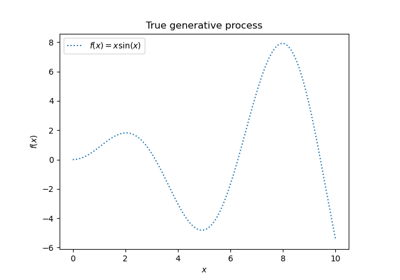
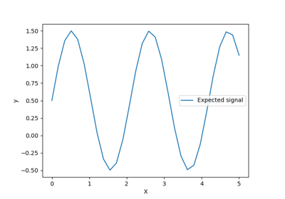
Comparison of kernel ridge and Gaussian process regression
Gaussian Processes regression: basic introductory example
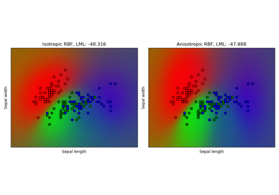
Gaussian process classification (GPC) on iris dataset

Gaussian process regression (GPR) on Mauna Loa CO2 data
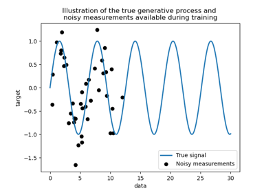
Gaussian process regression (GPR) with noise-level estimation
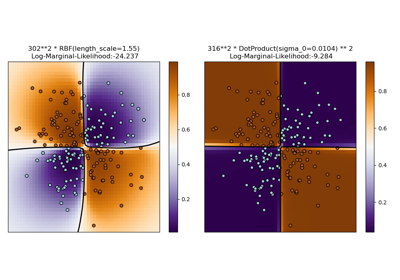
Illustration of Gaussian process classification (GPC) on the XOR dataset
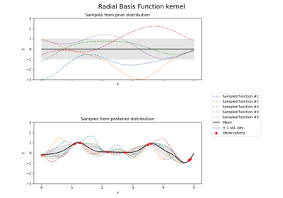
Illustration of prior and posterior Gaussian process for different kernels
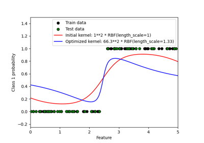
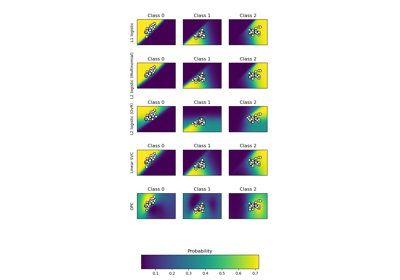
Probabilistic predictions with Gaussian process classification (GPC)