Note
Click here to download the full example code or to run this example in your browser via Binder
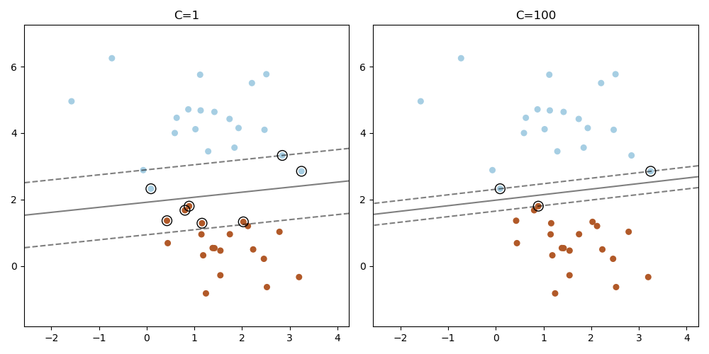
Plot the support vectors in LinearSVC
Unlike SVC (based on LIBSVM), LinearSVC (based on LIBLINEAR) does not provide the support vectors. This example demonstrates how to obtain the support vectors in LinearSVC.
import numpy as np
import matplotlib.pyplot as plt
from sklearn.datasets import make_blobs
from sklearn.svm import LinearSVC
from sklearn.inspection import DecisionBoundaryDisplay

X, y = make_blobs(n_samples=40, centers=2, random_state=0)

plt.figure(figsize=(10, 5))
for i, C in enumerate([1, 100]):
    # "hinge" is the standard SVM loss
    clf = LinearSVC(C=C, loss="hinge", random_state=42).fit(X, y)
    # obtain the support vectors through the decision function
    decision_function = clf.decision_function(X)
    # we can also calculate the decision function manually
    # decision_function = np.dot(X, clf.coef_[0]) + clf.intercept_[0]
    # The support vectors are the samples that lie within the margin
    # boundaries, whose size is conventionally constrained to 1
    support_vector_indices = np.where(np.abs(decision_function) <= 1 + 1e-15)[0]
    support_vectors = X[support_vector_indices]

    plt.subplot(1, 2, i + 1)
    plt.scatter(X[:, 0], X[:, 1], c=y, s=30, cmap=plt.cm.Paired)
    ax = plt.gca()
    DecisionBoundaryDisplay.from_estimator(
        clf,
        X,
        ax=ax,
        grid_resolution=50,
        plot_method="contour",
        colors="k",
        levels=[-1, 0, 1],
        alpha=0.5,
        linestyles=["--", "-", "--"],
    )
    plt.scatter(
        support_vectors[:, 0],
        support_vectors[:, 1],
        s=100,
        linewidth=1,
        facecolors="none",
        edgecolors="k",
    )
    plt.title("C=" + str(C))
plt.tight_layout()
plt.show()
Total running time of the script: ( 0 minutes 0.119 seconds)