Successive Halving Iterations

This example illustrates how a successive halving search (HalvingGridSearchCV and HalvingRandomSearchCV) iteratively chooses the best parameter combination out of multiple candidates.

import pandas as pd
from sklearn import datasets
import matplotlib.pyplot as plt
from scipy.stats import randint
import numpy as np

from sklearn.experimental import enable_halving_search_cv  # noqa
from sklearn.model_selection import HalvingRandomSearchCV
from sklearn.ensemble import RandomForestClassifier

We first define the parameter space and train a HalvingRandomSearchCV instance.

rng = np.random.RandomState(0)

X, y = datasets.make_classification(n_samples=400, n_features=12, random_state=rng)

clf = RandomForestClassifier(n_estimators=20, random_state=rng)

param_dist = {
    "max_depth": [3, None],
    "max_features": randint(1, 6),
    "min_samples_split": randint(2, 11),
    "bootstrap": [True, False],
    "criterion": ["gini", "entropy"],
}

rsh = HalvingRandomSearchCV(
    estimator=clf, param_distributions=param_dist, factor=2, random_state=rng
)
rsh.fit(X, y)

HalvingRandomSearchCV(estimator=RandomForestClassifier(n_estimators=20,
                                                       random_state=RandomState(MT19937) at 0x7F6E7E761B40),
                      factor=2,
                      param_distributions={'bootstrap': [True, False],
                                           'criterion': ['gini', 'entropy'],
                                           'max_depth': [3, None],
                                           'max_features': <scipy.stats._distn_infrastructure.rv_discrete_frozen object at 0x7f6e7e41fc10>,
                                           'min_samples_split': <scipy.stats._distn_infrastructure.rv_discrete_frozen object at 0x7f6dea2acdf0>},
                      random_state=RandomState(MT19937) at 0x7F6E7E761B40)

In a Jupyter environment, please rerun this cell to show the HTML representation or trust the notebook.
On GitHub, the HTML representation is unable to render, please try loading this page with nbviewer.org.

We can now use the cv_results_ attribute of the search estimator to inspect and plot the evolution of the search.

results = pd.DataFrame(rsh.cv_results_)
results["params_str"] = results.params.apply(str)
results.drop_duplicates(subset=("params_str", "iter"), inplace=True)
mean_scores = results.pivot(
    index="iter", columns="params_str", values="mean_test_score"
)
ax = mean_scores.plot(legend=False, alpha=0.6)

labels = [
    f"iter={i}\nn_samples={rsh.n_resources_[i]}\nn_candidates={rsh.n_candidates_[i]}"
    for i in range(rsh.n_iterations_)
]

ax.set_xticks(range(rsh.n_iterations_))
ax.set_xticklabels(labels, rotation=45, multialignment="left")
ax.set_title("Scores of candidates over iterations")
ax.set_ylabel("mean test score", fontsize=15)
ax.set_xlabel("iterations", fontsize=15)
plt.tight_layout()
plt.show()

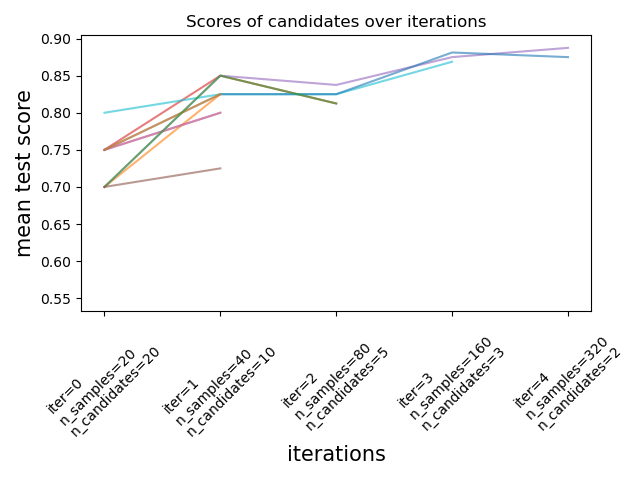
Number of candidates and amount of resource at each iteration

At the first iteration, a small amount of resources is used. The resource here is the number of samples that the estimators are trained on. All candidates are evaluated.

At the second iteration, only the best half of the candidates is evaluated. The number of allocated resources is doubled: candidates are evaluated on twice as many samples.

This process is repeated until the last iteration, where only 2 candidates are left. The best candidate is the candidate that has the best score at the last iteration.