This is documentation for an old release of Scikit-learn (version 1.1). Try the latest stable release (version 1.6) or development (unstable) versions.

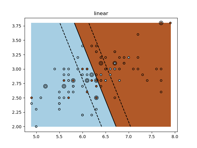
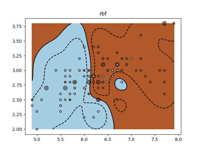
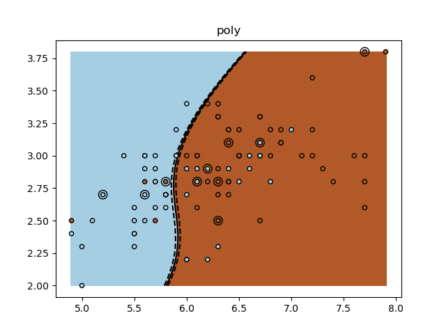
SVM Exercise

A tutorial exercise for using different SVM kernels.

This exercise is used in the Using kernels part of the Supervised learning: predicting an output variable from high-dimensional observations section of the A tutorial on statistical-learning for scientific data processing.

• 
• 
• 

import numpy as np
import matplotlib.pyplot as plt
from sklearn import datasets, svm

iris = datasets.load_iris()
X = iris.data
y = iris.target

X = X[y != 0, :2]
y = y[y != 0]

n_sample = len(X)

np.random.seed(0)
order = np.random.permutation(n_sample)
X = X[order]
y = y[order].astype(float)

X_train = X[: int(0.9 * n_sample)]
y_train = y[: int(0.9 * n_sample)]
X_test = X[int(0.9 * n_sample) :]
y_test = y[int(0.9 * n_sample) :]

# fit the model
for kernel in ("linear", "rbf", "poly"):
    clf = svm.SVC(kernel=kernel, gamma=10)
    clf.fit(X_train, y_train)

    plt.figure()
    plt.clf()
    plt.scatter(
        X[:, 0], X[:, 1], c=y, zorder=10, cmap=plt.cm.Paired, edgecolor="k", s=20
    )

    # Circle out the test data
    plt.scatter(
        X_test[:, 0], X_test[:, 1], s=80, facecolors="none", zorder=10, edgecolor="k"
    )

    plt.axis("tight")
    x_min = X[:, 0].min()
    x_max = X[:, 0].max()
    y_min = X[:, 1].min()
    y_max = X[:, 1].max()

    XX, YY = np.mgrid[x_min:x_max:200j, y_min:y_max:200j]
    Z = clf.decision_function(np.c_[XX.ravel(), YY.ravel()])

    # Put the result into a color plot
    Z = Z.reshape(XX.shape)
    plt.pcolormesh(XX, YY, Z > 0, cmap=plt.cm.Paired)
    plt.contour(
        XX,
        YY,
        Z,
        colors=["k", "k", "k"],
        linestyles=["--", "-", "--"],
        levels=[-0.5, 0, 0.5],
    )

    plt.title(kernel)
plt.show()