Post pruning decision trees with cost complexity pruning

The DecisionTreeClassifier provides parameters such as min_samples_leaf and max_depth to prevent a tree from overfiting. Cost complexity pruning provides another option to control the size of a tree. In DecisionTreeClassifier, this pruning technique is parameterized by the cost complexity parameter, ccp_alpha. Greater values of ccp_alpha increase the number of nodes pruned. Here we only show the effect of ccp_alpha on regularizing the trees and how to choose a ccp_alpha based on validation scores.

See also Minimal Cost-Complexity Pruning for details on pruning.

import matplotlib.pyplot as plt
from sklearn.model_selection import train_test_split
from sklearn.datasets import load_breast_cancer
from sklearn.tree import DecisionTreeClassifier

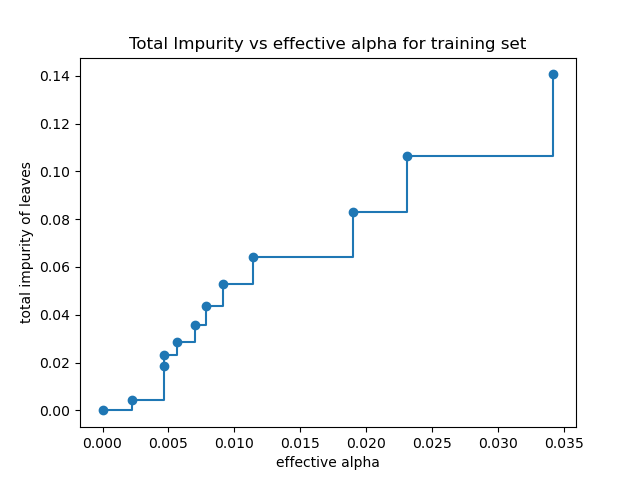
Total impurity of leaves vs effective alphas of pruned tree

Minimal cost complexity pruning recursively finds the node with the “weakest link”. The weakest link is characterized by an effective alpha, where the nodes with the smallest effective alpha are pruned first. To get an idea of what values of ccp_alpha could be appropriate, scikit-learn provides DecisionTreeClassifier.cost_complexity_pruning_path that returns the effective alphas and the corresponding total leaf impurities at each step of the pruning process. As alpha increases, more of the tree is pruned, which increases the total impurity of its leaves.

X, y = load_breast_cancer(return_X_y=True)
X_train, X_test, y_train, y_test = train_test_split(X, y, random_state=0)

clf = DecisionTreeClassifier(random_state=0)
path = clf.cost_complexity_pruning_path(X_train, y_train)
ccp_alphas, impurities = path.ccp_alphas, path.impurities

In the following plot, the maximum effective alpha value is removed, because it is the trivial tree with only one node.

fig, ax = plt.subplots()
ax.plot(ccp_alphas[:-1], impurities[:-1], marker="o", drawstyle="steps-post")
ax.set_xlabel("effective alpha")
ax.set_ylabel("total impurity of leaves")
ax.set_title("Total Impurity vs effective alpha for training set")

Out:

Text(0.5, 1.0, 'Total Impurity vs effective alpha for training set')

Next, we train a decision tree using the effective alphas. The last value in ccp_alphas is the alpha value that prunes the whole tree, leaving the tree, clfs[-1], with one node.

clfs = []
for ccp_alpha in ccp_alphas:
    clf = DecisionTreeClassifier(random_state=0, ccp_alpha=ccp_alpha)
    clf.fit(X_train, y_train)
    clfs.append(clf)
print(
    "Number of nodes in the last tree is: {} with ccp_alpha: {}".format(
        clfs[-1].tree_.node_count, ccp_alphas[-1]
    )
)

Out:

Number of nodes in the last tree is: 1 with ccp_alpha: 0.3272984419327777

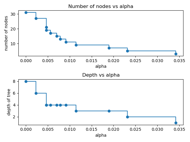
For the remainder of this example, we remove the last element in clfs and ccp_alphas, because it is the trivial tree with only one node. Here we show that the number of nodes and tree depth decreases as alpha increases.

clfs = clfs[:-1]
ccp_alphas = ccp_alphas[:-1]

node_counts = [clf.tree_.node_count for clf in clfs]
depth = [clf.tree_.max_depth for clf in clfs]
fig, ax = plt.subplots(2, 1)
ax[0].plot(ccp_alphas, node_counts, marker="o", drawstyle="steps-post")
ax[0].set_xlabel("alpha")
ax[0].set_ylabel("number of nodes")
ax[0].set_title("Number of nodes vs alpha")
ax[1].plot(ccp_alphas, depth, marker="o", drawstyle="steps-post")
ax[1].set_xlabel("alpha")
ax[1].set_ylabel("depth of tree")
ax[1].set_title("Depth vs alpha")
fig.tight_layout()

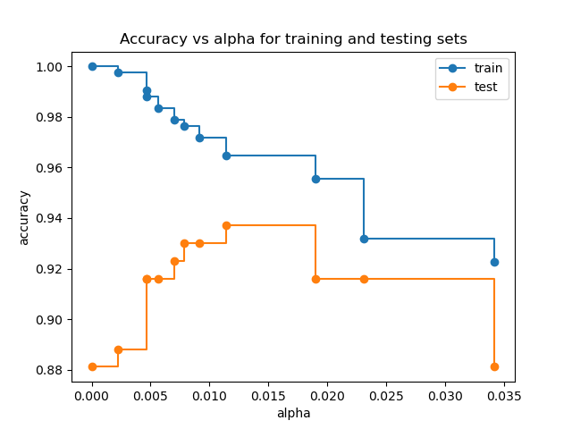
Accuracy vs alpha for training and testing sets

When ccp_alpha is set to zero and keeping the other default parameters of DecisionTreeClassifier, the tree overfits, leading to a 100% training accuracy and 88% testing accuracy. As alpha increases, more of the tree is pruned, thus creating a decision tree that generalizes better. In this example, setting ccp_alpha=0.015 maximizes the testing accuracy.

train_scores = [clf.score(X_train, y_train) for clf in clfs]
test_scores = [clf.score(X_test, y_test) for clf in clfs]

fig, ax = plt.subplots()
ax.set_xlabel("alpha")
ax.set_ylabel("accuracy")
ax.set_title("Accuracy vs alpha for training and testing sets")
ax.plot(ccp_alphas, train_scores, marker="o", label="train", drawstyle="steps-post")
ax.plot(ccp_alphas, test_scores, marker="o", label="test", drawstyle="steps-post")
ax.legend()
plt.show()