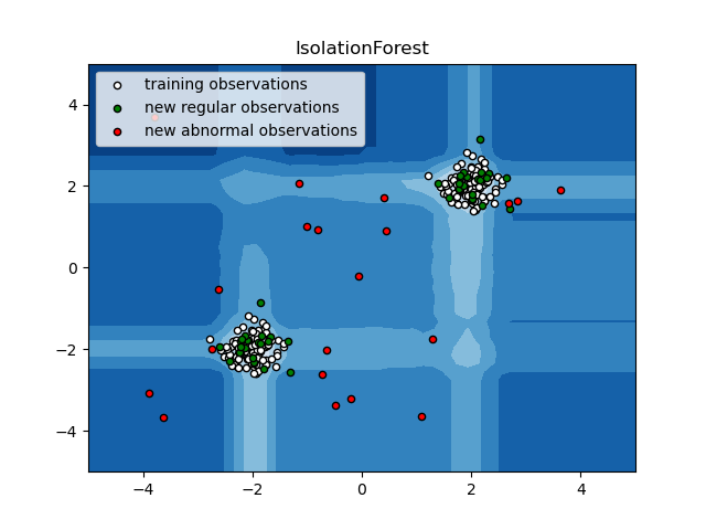
IsolationForest example

An example using IsolationForest for anomaly detection.

The IsolationForest ‘isolates’ observations by randomly selecting a feature and then randomly selecting a split value between the maximum and minimum values of the selected feature.

Since recursive partitioning can be represented by a tree structure, the number of splittings required to isolate a sample is equivalent to the path length from the root node to the terminating node.

This path length, averaged over a forest of such random trees, is a measure of normality and our decision function.

Random partitioning produces noticeable shorter paths for anomalies. Hence, when a forest of random trees collectively produce shorter path lengths for particular samples, they are highly likely to be anomalies.

import numpy as np
import matplotlib.pyplot as plt
from sklearn.ensemble import IsolationForest

rng = np.random.RandomState(42)

# Generate train data
X = 0.3 * rng.randn(100, 2)
X_train = np.r_[X + 2, X - 2]
# Generate some regular novel observations
X = 0.3 * rng.randn(20, 2)
X_test = np.r_[X + 2, X - 2]
# Generate some abnormal novel observations
X_outliers = rng.uniform(low=-4, high=4, size=(20, 2))

# fit the model
clf = IsolationForest(max_samples=100, random_state=rng)
clf.fit(X_train)
y_pred_train = clf.predict(X_train)
y_pred_test = clf.predict(X_test)
y_pred_outliers = clf.predict(X_outliers)

# plot the line, the samples, and the nearest vectors to the plane
xx, yy = np.meshgrid(np.linspace(-5, 5, 50), np.linspace(-5, 5, 50))
Z = clf.decision_function(np.c_[xx.ravel(), yy.ravel()])
Z = Z.reshape(xx.shape)

plt.title("IsolationForest")
plt.contourf(xx, yy, Z, cmap=plt.cm.Blues_r)

b1 = plt.scatter(X_train[:, 0], X_train[:, 1], c="white", s=20, edgecolor="k")
b2 = plt.scatter(X_test[:, 0], X_test[:, 1], c="green", s=20, edgecolor="k")
c = plt.scatter(X_outliers[:, 0], X_outliers[:, 1], c="red", s=20, edgecolor="k")
plt.axis("tight")
plt.xlim((-5, 5))
plt.ylim((-5, 5))
plt.legend(
    [b1, b2, c],
    ["training observations", "new regular observations", "new abnormal observations"],
    loc="upper left",
)
plt.show()