This is documentation for an old release of Scikit-learn (version 1.0). Try the latest stable release (version 1.6) or development (unstable) versions.

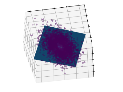
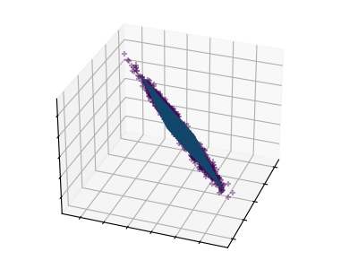
Principal components analysis (PCA)

These figures aid in illustrating how a point cloud can be very flat in one direction–which is where PCA comes in to choose a direction that is not flat.

• 
• 

Out:

/home/circleci/project/examples/decomposition/plot_pca_3d.py:60: MatplotlibDeprecationWarning: Axes3D(fig) adding itself to the figure is deprecated since 3.4. Pass the keyword argument auto_add_to_figure=False and use fig.add_axes(ax) to suppress this warning. The default value of auto_add_to_figure will change to False in mpl3.5 and True values will no longer work in 3.6.  This is consistent with other Axes classes.
  ax = Axes3D(fig, rect=[0, 0, 0.95, 1], elev=elev, azim=azim)
/home/circleci/project/examples/decomposition/plot_pca_3d.py:60: MatplotlibDeprecationWarning: Axes3D(fig) adding itself to the figure is deprecated since 3.4. Pass the keyword argument auto_add_to_figure=False and use fig.add_axes(ax) to suppress this warning. The default value of auto_add_to_figure will change to False in mpl3.5 and True values will no longer work in 3.6.  This is consistent with other Axes classes.
  ax = Axes3D(fig, rect=[0, 0, 0.95, 1], elev=elev, azim=azim)

# Authors: Gael Varoquaux
#          Jaques Grobler
#          Kevin Hughes
# License: BSD 3 clause

from sklearn.decomposition import PCA

from mpl_toolkits.mplot3d import Axes3D
import numpy as np
import matplotlib.pyplot as plt
from scipy import stats


# #############################################################################
# Create the data

e = np.exp(1)
np.random.seed(4)


def pdf(x):
    return 0.5 * (stats.norm(scale=0.25 / e).pdf(x) + stats.norm(scale=4 / e).pdf(x))


y = np.random.normal(scale=0.5, size=(30000))
x = np.random.normal(scale=0.5, size=(30000))
z = np.random.normal(scale=0.1, size=len(x))

density = pdf(x) * pdf(y)
pdf_z = pdf(5 * z)

density *= pdf_z

a = x + y
b = 2 * y
c = a - b + z

norm = np.sqrt(a.var() + b.var())
a /= norm
b /= norm


# #############################################################################
# Plot the figures
def plot_figs(fig_num, elev, azim):
    fig = plt.figure(fig_num, figsize=(4, 3))
    plt.clf()
    ax = Axes3D(fig, rect=[0, 0, 0.95, 1], elev=elev, azim=azim)

    ax.scatter(a[::10], b[::10], c[::10], c=density[::10], marker="+", alpha=0.4)
    Y = np.c_[a, b, c]

    # Using SciPy's SVD, this would be:
    # _, pca_score, Vt = scipy.linalg.svd(Y, full_matrices=False)

    pca = PCA(n_components=3)
    pca.fit(Y)
    V = pca.components_.T

    x_pca_axis, y_pca_axis, z_pca_axis = 3 * V
    x_pca_plane = np.r_[x_pca_axis[:2], -x_pca_axis[1::-1]]
    y_pca_plane = np.r_[y_pca_axis[:2], -y_pca_axis[1::-1]]
    z_pca_plane = np.r_[z_pca_axis[:2], -z_pca_axis[1::-1]]
    x_pca_plane.shape = (2, 2)
    y_pca_plane.shape = (2, 2)
    z_pca_plane.shape = (2, 2)
    ax.plot_surface(x_pca_plane, y_pca_plane, z_pca_plane)
    ax.w_xaxis.set_ticklabels([])
    ax.w_yaxis.set_ticklabels([])
    ax.w_zaxis.set_ticklabels([])


elev = -40
azim = -80
plot_figs(1, elev, azim)

elev = 30
azim = 20
plot_figs(2, elev, azim)

plt.show()