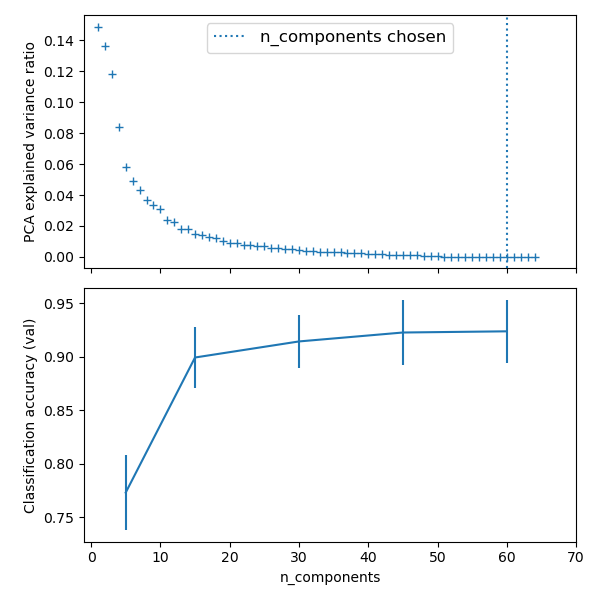
Pipelining: chaining a PCA and a logistic regression

The PCA does an unsupervised dimensionality reduction, while the logistic regression does the prediction.

We use a GridSearchCV to set the dimensionality of the PCA

Out:

Best parameter (CV score=0.924):
{'logistic__C': 0.046415888336127774, 'pca__n_components': 60}
/home/circleci/miniconda/envs/testenv/lib/python3.9/site-packages/pandas/core/indexes/base.py:6982: FutureWarning: In a future version, the Index constructor will not infer numeric dtypes when passed object-dtype sequences (matching Series behavior)
  return Index(sequences[0], name=names)

# Code source: Gaël Varoquaux
# Modified for documentation by Jaques Grobler
# License: BSD 3 clause

import numpy as np
import matplotlib.pyplot as plt
import pandas as pd

from sklearn import datasets
from sklearn.decomposition import PCA
from sklearn.linear_model import LogisticRegression
from sklearn.pipeline import Pipeline
from sklearn.model_selection import GridSearchCV
from sklearn.preprocessing import StandardScaler

# Define a pipeline to search for the best combination of PCA truncation
# and classifier regularization.
pca = PCA()
# Define a Standard Scaler to normalize inputs
scaler = StandardScaler()

# set the tolerance to a large value to make the example faster
logistic = LogisticRegression(max_iter=10000, tol=0.1)
pipe = Pipeline(steps=[("scaler", scaler), ("pca", pca), ("logistic", logistic)])

X_digits, y_digits = datasets.load_digits(return_X_y=True)
# Parameters of pipelines can be set using ‘__’ separated parameter names:
param_grid = {
    "pca__n_components": [5, 15, 30, 45, 60],
    "logistic__C": np.logspace(-4, 4, 4),
}
search = GridSearchCV(pipe, param_grid, n_jobs=2)
search.fit(X_digits, y_digits)
print("Best parameter (CV score=%0.3f):" % search.best_score_)
print(search.best_params_)

# Plot the PCA spectrum
pca.fit(X_digits)

fig, (ax0, ax1) = plt.subplots(nrows=2, sharex=True, figsize=(6, 6))
ax0.plot(
    np.arange(1, pca.n_components_ + 1), pca.explained_variance_ratio_, "+", linewidth=2
)
ax0.set_ylabel("PCA explained variance ratio")

ax0.axvline(
    search.best_estimator_.named_steps["pca"].n_components,
    linestyle=":",
    label="n_components chosen",
)
ax0.legend(prop=dict(size=12))

# For each number of components, find the best classifier results
results = pd.DataFrame(search.cv_results_)
components_col = "param_pca__n_components"
best_clfs = results.groupby(components_col).apply(
    lambda g: g.nlargest(1, "mean_test_score")
)

best_clfs.plot(
    x=components_col, y="mean_test_score", yerr="std_test_score", legend=False, ax=ax1
)
ax1.set_ylabel("Classification accuracy (val)")
ax1.set_xlabel("n_components")

plt.xlim(-1, 70)

plt.tight_layout()
plt.show()