Note
Click here to download the full example code or to run this example in your browser via Binder
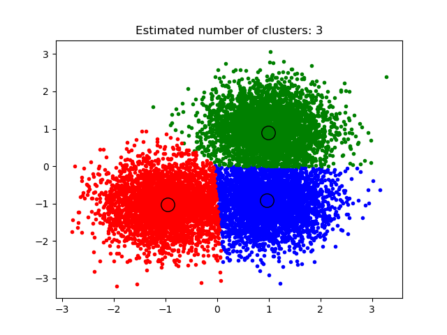
A demo of the mean-shift clustering algorithm
Reference:
Dorin Comaniciu and Peter Meer, “Mean Shift: A robust approach toward feature space analysis”. IEEE Transactions on Pattern Analysis and Machine Intelligence. 2002. pp. 603-619.
Out:
number of estimated clusters : 3
print(__doc__)

import numpy as np
from sklearn.cluster import MeanShift, estimate_bandwidth
from sklearn.datasets import make_blobs

# #############################################################################
# Generate sample data
centers = [[1, 1], [-1, -1], [1, -1]]
X, _ = make_blobs(n_samples=10000, centers=centers, cluster_std=0.6)

# #############################################################################
# Compute clustering with MeanShift

# The following bandwidth can be automatically detected using
bandwidth = estimate_bandwidth(X, quantile=0.2, n_samples=500)

ms = MeanShift(bandwidth=bandwidth, bin_seeding=True)
ms.fit(X)
labels = ms.labels_
cluster_centers = ms.cluster_centers_

labels_unique = np.unique(labels)
n_clusters_ = len(labels_unique)

print("number of estimated clusters : %d" % n_clusters_)

# #############################################################################
# Plot result
import matplotlib.pyplot as plt
from itertools import cycle

plt.figure(1)
plt.clf()

colors = cycle('bgrcmykbgrcmykbgrcmykbgrcmyk')
for k, col in zip(range(n_clusters_), colors):
    my_members = labels == k
    cluster_center = cluster_centers[k]
    plt.plot(X[my_members, 0], X[my_members, 1], col + '.')
    plt.plot(cluster_center[0], cluster_center[1], 'o', markerfacecolor=col,
             markeredgecolor='k', markersize=14)
plt.title('Estimated number of clusters: %d' % n_clusters_)
plt.show()
Total running time of the script: ( 0 minutes 0.514 seconds)