SVM: Weighted samples

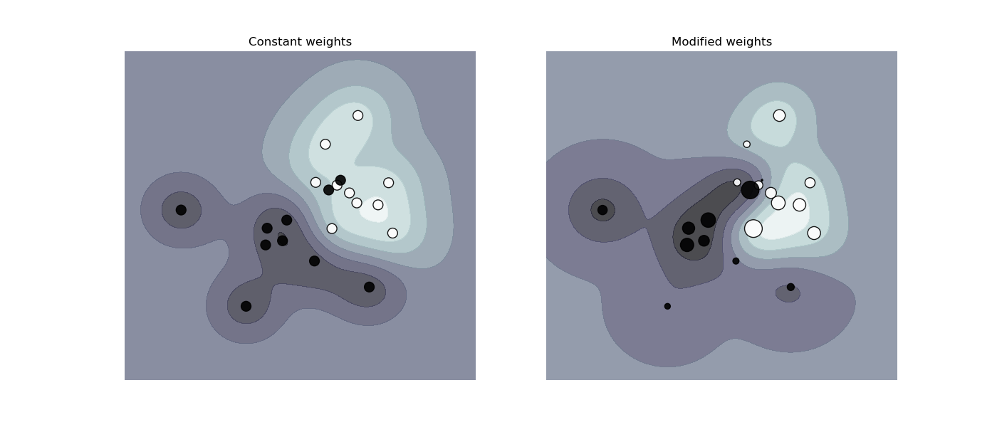
Plot decision function of a weighted dataset, where the size of points is proportional to its weight.

The sample weighting rescales the C parameter, which means that the classifier puts more emphasis on getting these points right. The effect might often be subtle. To emphasize the effect here, we particularly weight outliers, making the deformation of the decision boundary very visible.

print(__doc__)

import numpy as np
import matplotlib.pyplot as plt
from sklearn import svm


def plot_decision_function(classifier, sample_weight, axis, title):
    # plot the decision function
    xx, yy = np.meshgrid(np.linspace(-4, 5, 500), np.linspace(-4, 5, 500))

    Z = classifier.decision_function(np.c_[xx.ravel(), yy.ravel()])
    Z = Z.reshape(xx.shape)

    # plot the line, the points, and the nearest vectors to the plane
    axis.contourf(xx, yy, Z, alpha=0.75, cmap=plt.cm.bone)
    axis.scatter(X[:, 0], X[:, 1], c=y, s=100 * sample_weight, alpha=0.9,
                 cmap=plt.cm.bone, edgecolors='black')

    axis.axis('off')
    axis.set_title(title)


# we create 20 points
np.random.seed(0)
X = np.r_[np.random.randn(10, 2) + [1, 1], np.random.randn(10, 2)]
y = [1] * 10 + [-1] * 10
sample_weight_last_ten = abs(np.random.randn(len(X)))
sample_weight_constant = np.ones(len(X))
# and bigger weights to some outliers
sample_weight_last_ten[15:] *= 5
sample_weight_last_ten[9] *= 15

# for reference, first fit without sample weights

# fit the model
clf_weights = svm.SVC(gamma=1)
clf_weights.fit(X, y, sample_weight=sample_weight_last_ten)

clf_no_weights = svm.SVC(gamma=1)
clf_no_weights.fit(X, y)

fig, axes = plt.subplots(1, 2, figsize=(14, 6))
plot_decision_function(clf_no_weights, sample_weight_constant, axes[0],
                       "Constant weights")
plot_decision_function(clf_weights, sample_weight_last_ten, axes[1],
                       "Modified weights")

plt.show()

Total running time of the script: ( 0 minutes 0.349 seconds)