This is documentation for an old release of Scikit-learn (version 0.21). Try the latest stable release (version 1.6) or development (unstable) versions.

This is documentation for an old release of Scikit-learn (version 0.21). Try the latest stable release (version 1.6) or development (unstable) versions.

Neighborhood Components Analysis Illustration

An example illustrating the goal of learning a distance metric that maximizes the nearest neighbors classification accuracy. The example is solely for illustration purposes. Please refer to the User Guide for more information.

• 
• 

# License: BSD 3 clause

import numpy as np
import matplotlib.pyplot as plt
from sklearn.datasets import make_classification
from sklearn.neighbors import NeighborhoodComponentsAnalysis
from matplotlib import cm
from sklearn.utils.fixes import logsumexp

print(__doc__)

n_neighbors = 1
random_state = 0

# Create a tiny data set of 9 samples from 3 classes
X, y = make_classification(n_samples=9, n_features=2, n_informative=2,
                           n_redundant=0, n_classes=3, n_clusters_per_class=1,
                           class_sep=1.0, random_state=random_state)

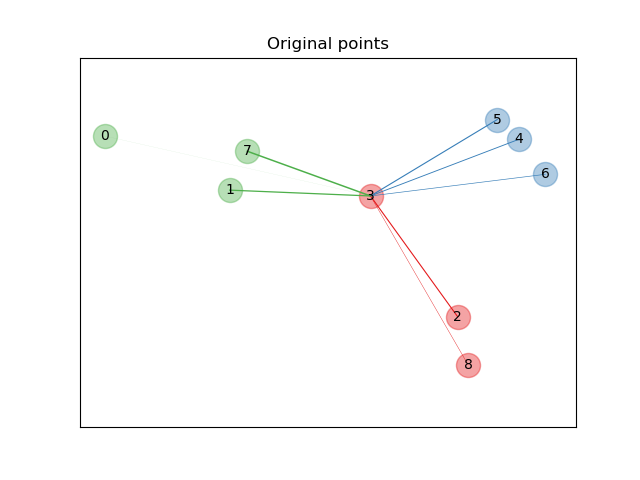
# Plot the points in the original space
plt.figure()
ax = plt.gca()

# Draw the graph nodes
for i in range(X.shape[0]):
    ax.text(X[i, 0], X[i, 1], str(i), va='center', ha='center')
    ax.scatter(X[i, 0], X[i, 1], s=300, c=cm.Set1(y[i]), alpha=0.4)


def p_i(X, i):
    diff_embedded = X[i] - X
    dist_embedded = np.einsum('ij,ij->i', diff_embedded,
                              diff_embedded)
    dist_embedded[i] = np.inf

    # compute exponentiated distances (use the log-sum-exp trick to
    # avoid numerical instabilities
    exp_dist_embedded = np.exp(-dist_embedded -
                               logsumexp(-dist_embedded))
    return exp_dist_embedded


def relate_point(X, i, ax):
    pt_i = X[i]
    for j, pt_j in enumerate(X):
        thickness = p_i(X, i)
        if i != j:
            line = ([pt_i[0], pt_j[0]], [pt_i[1], pt_j[1]])
            ax.plot(*line, c=cm.Set1(y[j]),
                    linewidth=5*thickness[j])


# we consider only point 3
i = 3

# Plot bonds linked to sample i in the original space
relate_point(X, i, ax)
ax.set_title("Original points")
ax.axes.get_xaxis().set_visible(False)
ax.axes.get_yaxis().set_visible(False)
ax.axis('equal')

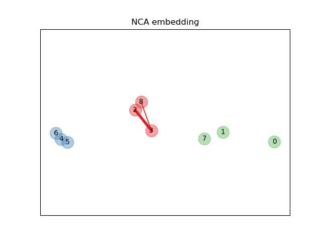
# Learn an embedding with NeighborhoodComponentsAnalysis
nca = NeighborhoodComponentsAnalysis(max_iter=30, random_state=random_state)
nca = nca.fit(X, y)

# Plot the points after transformation with NeighborhoodComponentsAnalysis
plt.figure()
ax2 = plt.gca()

# Get the embedding and find the new nearest neighbors
X_embedded = nca.transform(X)

relate_point(X_embedded, i, ax2)

for i in range(len(X)):
    ax2.text(X_embedded[i, 0], X_embedded[i, 1], str(i),
             va='center', ha='center')
    ax2.scatter(X_embedded[i, 0], X_embedded[i, 1], s=300, c=cm.Set1(y[i]),
                alpha=0.4)

# Make axes equal so that boundaries are displayed correctly as circles
ax2.set_title("NCA embedding")
ax2.axes.get_xaxis().set_visible(False)
ax2.axes.get_yaxis().set_visible(False)
ax2.axis('equal')
plt.show()

Total running time of the script: ( 0 minutes 0.069 seconds)