sklearn.isotonic.IsotonicRegression

class sklearn.isotonic.IsotonicRegression(y_min=None, y_max=None, increasing=True, out_of_bounds='nan')

Isotonic regression model.

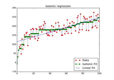
The isotonic regression optimization problem is defined by:

min sum w_i (y[i] - y_[i]) ** 2

subject to y_[i] <= y_[j] whenever X[i] <= X[j]
and min(y_) = y_min, max(y_) = y_max

where:

• y[i] are inputs (real numbers)
• y_[i] are fitted
• X specifies the order. If X is non-decreasing then y_ is non-decreasing.
• w[i] are optional strictly positive weights (default to 1.0)

Read more in the User Guide.

Parameters:

y_min : optional, default: None

If not None, set the lowest value of the fit to y_min.

y_max : optional, default: None

If not None, set the highest value of the fit to y_max.

increasing : boolean or string, optional, default: True

If boolean, whether or not to fit the isotonic regression with y increasing or decreasing.

The string value “auto” determines whether y should increase or decrease based on the Spearman correlation estimate’s sign.

out_of_bounds : string, optional, default: “nan”

The out_of_bounds parameter handles how x-values outside of the training domain are handled. When set to “nan”, predicted y-values will be NaN. When set to “clip”, predicted y-values will be set to the value corresponding to the nearest train interval endpoint. When set to “raise”, allow interp1d to throw ValueError.

Attributes:

X_ : ndarray (n_samples, )

A copy of the input X.

y_ : ndarray (n_samples, )

Isotonic fit of y.

X_min_ : float

Minimum value of input array X_ for left bound.

X_max_ : float

Maximum value of input array X_ for right bound.

f_ : function

The stepwise interpolating function that covers the domain X_.

Notes

Ties are broken using the secondary method from Leeuw, 1977.

References

Isotonic Median Regression: A Linear Programming Approach Nilotpal Chakravarti Mathematics of Operations Research Vol. 14, No. 2 (May, 1989), pp. 303-308

Isotone Optimization in R : Pool-Adjacent-Violators Algorithm (PAVA) and Active Set Methods Leeuw, Hornik, Mair Journal of Statistical Software 2009

Correctness of Kruskal’s algorithms for monotone regression with ties Leeuw, Psychometrica, 1977

Methods

fit(X, y[, sample_weight])	Fit the model using X, y as training data.
fit_transform(X[, y])	Fit to data, then transform it.
get_params([deep])	Get parameters for this estimator.
predict(T)	Predict new data by linear interpolation.
score(X, y[, sample_weight])	Returns the coefficient of determination R^2 of the prediction.
set_params(**params)	Set the parameters of this estimator.
transform(T)	Transform new data by linear interpolation

__init__(y_min=None, y_max=None, increasing=True, out_of_bounds='nan')

fit(X, y, sample_weight=None)

Fit the model using X, y as training data.

Parameters:

X : array-like, shape=(n_samples,)

Training data.

y : array-like, shape=(n_samples,)

Training target.

sample_weight : array-like, shape=(n_samples,), optional, default: None

Weights. If set to None, all weights will be set to 1 (equal weights).

Returns:

self : object

Returns an instance of self.

Notes

X is stored for future use, as transform needs X to interpolate new input data.

fit_transform(X, y=None, **fit_params)

Fit to data, then transform it.

Fits transformer to X and y with optional parameters fit_params and returns a transformed version of X.

Parameters:

X : numpy array of shape [n_samples, n_features]

Training set.

y : numpy array of shape [n_samples]

Target values.

Returns:

X_new : numpy array of shape [n_samples, n_features_new]

Transformed array.

get_params(deep=True)

Get parameters for this estimator.

Parameters:

deep: boolean, optional :

If True, will return the parameters for this estimator and contained subobjects that are estimators.

Returns:

params : mapping of string to any

Parameter names mapped to their values.

predict(T)

Predict new data by linear interpolation.

Parameters:

T : array-like, shape=(n_samples,)

Data to transform.

Returns:

T_ : array, shape=(n_samples,)

Transformed data.

score(X, y, sample_weight=None)

Returns the coefficient of determination R^2 of the prediction.

The coefficient R^2 is defined as (1 - u/v), where u is the regression sum of squares ((y_true - y_pred) ** 2).sum() and v is the residual sum of squares ((y_true - y_true.mean()) ** 2).sum(). Best possible score is 1.0 and it can be negative (because the model can be arbitrarily worse). A constant model that always predicts the expected value of y, disregarding the input features, would get a R^2 score of 0.0.

Parameters:

X : array-like, shape = (n_samples, n_features)

Test samples.

y : array-like, shape = (n_samples) or (n_samples, n_outputs)

True values for X.

sample_weight : array-like, shape = [n_samples], optional

Sample weights.

Returns:

score : float

R^2 of self.predict(X) wrt. y.

set_params(**params)

Set the parameters of this estimator.

The method works on simple estimators as well as on nested objects (such as pipelines). The former have parameters of the form <component>__<parameter> so that it’s possible to update each component of a nested object.

Returns:self :

transform(T)

Transform new data by linear interpolation

Parameters:

T : array-like, shape=(n_samples,)

Data to transform.

Returns:

T_ : array, shape=(n_samples,)

The transformed data

Examples using sklearn.isotonic.IsotonicRegression

Isotonic Regression