GMM classification

Demonstration of Gaussian mixture models for classification.

See Gaussian mixture models for more information on the estimator.

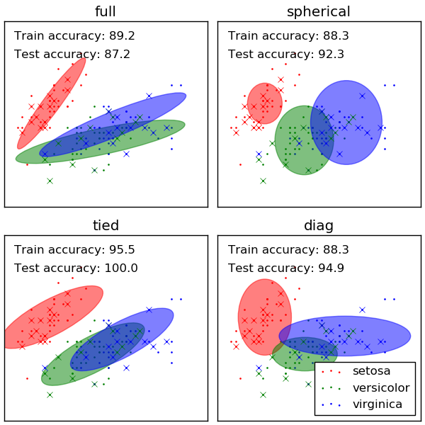
Plots predicted labels on both training and held out test data using a variety of GMM classifiers on the iris dataset.

Compares GMMs with spherical, diagonal, full, and tied covariance matrices in increasing order of performance. Although one would expect full covariance to perform best in general, it is prone to overfitting on small datasets and does not generalize well to held out test data.

On the plots, train data is shown as dots, while test data is shown as crosses. The iris dataset is four-dimensional. Only the first two dimensions are shown here, and thus some points are separated in other dimensions.

Python source code: plot_gmm_classifier.py

print(__doc__)

# Author: Ron Weiss <ronweiss@gmail.com>, Gael Varoquaux
# License: BSD 3 clause

# $Id$

import matplotlib.pyplot as plt
import matplotlib as mpl
import numpy as np

from sklearn import datasets
from sklearn.cross_validation import StratifiedKFold
from sklearn.externals.six.moves import xrange
from sklearn.mixture import GMM


def make_ellipses(gmm, ax):
    for n, color in enumerate('rgb'):
        v, w = np.linalg.eigh(gmm._get_covars()[n][:2, :2])
        u = w[0] / np.linalg.norm(w[0])
        angle = np.arctan2(u[1], u[0])
        angle = 180 * angle / np.pi  # convert to degrees
        v *= 9
        ell = mpl.patches.Ellipse(gmm.means_[n, :2], v[0], v[1],
                                  180 + angle, color=color)
        ell.set_clip_box(ax.bbox)
        ell.set_alpha(0.5)
        ax.add_artist(ell)

iris = datasets.load_iris()

# Break up the dataset into non-overlapping training (75%) and testing
# (25%) sets.
skf = StratifiedKFold(iris.target, n_folds=4)
# Only take the first fold.
train_index, test_index = next(iter(skf))


X_train = iris.data[train_index]
y_train = iris.target[train_index]
X_test = iris.data[test_index]
y_test = iris.target[test_index]

n_classes = len(np.unique(y_train))

# Try GMMs using different types of covariances.
classifiers = dict((covar_type, GMM(n_components=n_classes,
                    covariance_type=covar_type, init_params='wc', n_iter=20))
                   for covar_type in ['spherical', 'diag', 'tied', 'full'])

n_classifiers = len(classifiers)

plt.figure(figsize=(3 * n_classifiers / 2, 6))
plt.subplots_adjust(bottom=.01, top=0.95, hspace=.15, wspace=.05,
                    left=.01, right=.99)


for index, (name, classifier) in enumerate(classifiers.items()):
    # Since we have class labels for the training data, we can
    # initialize the GMM parameters in a supervised manner.
    classifier.means_ = np.array([X_train[y_train == i].mean(axis=0)
                                  for i in xrange(n_classes)])

    # Train the other parameters using the EM algorithm.
    classifier.fit(X_train)

    h = plt.subplot(2, n_classifiers / 2, index + 1)
    make_ellipses(classifier, h)

    for n, color in enumerate('rgb'):
        data = iris.data[iris.target == n]
        plt.scatter(data[:, 0], data[:, 1], 0.8, color=color,
                    label=iris.target_names[n])
    # Plot the test data with crosses
    for n, color in enumerate('rgb'):
        data = X_test[y_test == n]
        plt.plot(data[:, 0], data[:, 1], 'x', color=color)

    y_train_pred = classifier.predict(X_train)
    train_accuracy = np.mean(y_train_pred.ravel() == y_train.ravel()) * 100
    plt.text(0.05, 0.9, 'Train accuracy: %.1f' % train_accuracy,
             transform=h.transAxes)

    y_test_pred = classifier.predict(X_test)
    test_accuracy = np.mean(y_test_pred.ravel() == y_test.ravel()) * 100
    plt.text(0.05, 0.8, 'Test accuracy: %.1f' % test_accuracy,
             transform=h.transAxes)

    plt.xticks(())
    plt.yticks(())
    plt.title(name)

plt.legend(loc='lower right', prop=dict(size=12))


plt.show()

Total running time of the example: 0.43 seconds ( 0 minutes 0.43 seconds)