
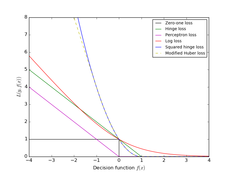
SGD: convex loss functions
A plot that compares the various convex loss functions supported by
sklearn.linear_model.SGDClassifier .
Python source code: plot_sgd_loss_functions.py
print(__doc__)

import numpy as np
import matplotlib.pyplot as plt


def modified_huber_loss(y_true, y_pred):
    z = y_pred * y_true
    loss = -4 * z
    loss[z >= -1] = (1 - z[z >= -1]) ** 2
    loss[z >= 1.] = 0
    return loss


xmin, xmax = -4, 4
xx = np.linspace(xmin, xmax, 100)
plt.plot([xmin, 0, 0, xmax], [1, 1, 0, 0], 'k-',
         label="Zero-one loss")
plt.plot(xx, np.where(xx < 1, 1 - xx, 0), 'g-',
         label="Hinge loss")
plt.plot(xx, -np.minimum(xx, 0), 'm-',
         label="Perceptron loss")
plt.plot(xx, np.log2(1 + np.exp(-xx)), 'r-',
         label="Log loss")
plt.plot(xx, np.where(xx < 1, 1 - xx, 0) ** 2, 'b-',
         label="Squared hinge loss")
plt.plot(xx, modified_huber_loss(xx, 1), 'y--',
         label="Modified Huber loss")
plt.ylim((0, 8))
plt.legend(loc="upper right")
plt.xlabel(r"Decision function $f(x)$")
plt.ylabel("$L(y, f(x))$")
plt.show()
Total running time of the example: 0.08 seconds ( 0 minutes 0.08 seconds)