Lasso and Elastic Net¶

Lasso and elastic net (L1 and L2 penalisation) implemented using a coordinate descent.

The coefficients can be forced to be positive.

Script output:

Computing regularization path using the lasso...
Computing regularization path using the positive lasso...
Computing regularization path using the elastic net...
Computing regularization path using the positve elastic net...

Python source code: plot_lasso_coordinate_descent_path.py

print(__doc__)

# Author: Alexandre Gramfort <alexandre.gramfort@inria.fr>
# License: BSD 3 clause

import numpy as np
import matplotlib.pyplot as plt

from sklearn.linear_model import lasso_path, enet_path
from sklearn import datasets

diabetes = datasets.load_diabetes()
X = diabetes.data
y = diabetes.target

X /= X.std(axis=0)  # Standardize data (easier to set the l1_ratio parameter)

# Compute paths

eps = 5e-3  # the smaller it is the longer is the path

print("Computing regularization path using the lasso...")
alphas_lasso, coefs_lasso, _ = lasso_path(X, y, eps, fit_intercept=False)

print("Computing regularization path using the positive lasso...")
alphas_positive_lasso, coefs_positive_lasso, _ = lasso_path(
    X, y, eps, positive=True, fit_intercept=False)
print("Computing regularization path using the elastic net...")
alphas_enet, coefs_enet, _ = enet_path(
    X, y, eps=eps, l1_ratio=0.8, fit_intercept=False)

print("Computing regularization path using the positve elastic net...")
alphas_positive_enet, coefs_positive_enet, _ = enet_path(
    X, y, eps=eps, l1_ratio=0.8, positive=True, fit_intercept=False)

# Display results

plt.figure(1)
ax = plt.gca()
ax.set_color_cycle(2 * ['b', 'r', 'g', 'c', 'k'])
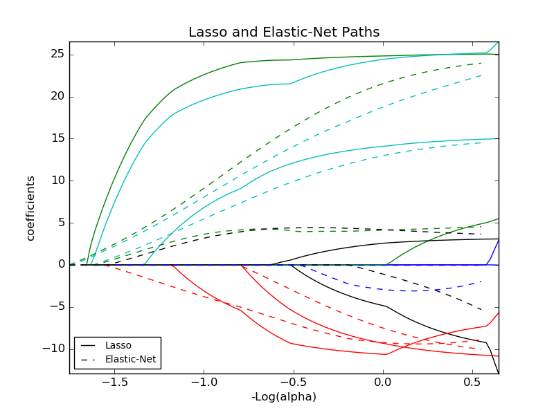
l1 = plt.plot(-np.log10(alphas_lasso), coefs_lasso.T)
l2 = plt.plot(-np.log10(alphas_enet), coefs_enet.T, linestyle='--')

plt.xlabel('-Log(alpha)')
plt.ylabel('coefficients')
plt.title('Lasso and Elastic-Net Paths')
plt.legend((l1[-1], l2[-1]), ('Lasso', 'Elastic-Net'), loc='lower left')
plt.axis('tight')


plt.figure(2)
ax = plt.gca()
ax.set_color_cycle(2 * ['b', 'r', 'g', 'c', 'k'])
l1 = plt.plot(-np.log10(alphas_lasso), coefs_lasso.T)
l2 = plt.plot(-np.log10(alphas_positive_lasso), coefs_positive_lasso.T,
              linestyle='--')

plt.xlabel('-Log(alpha)')
plt.ylabel('coefficients')
plt.title('Lasso and positive Lasso')
plt.legend((l1[-1], l2[-1]), ('Lasso', 'positive Lasso'), loc='lower left')
plt.axis('tight')


plt.figure(3)
ax = plt.gca()
ax.set_color_cycle(2 * ['b', 'r', 'g', 'c', 'k'])
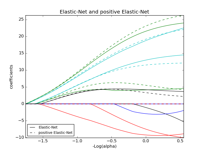
l1 = plt.plot(-np.log10(alphas_enet), coefs_enet.T)
l2 = plt.plot(-np.log10(alphas_positive_enet), coefs_positive_enet.T,
              linestyle='--')

plt.xlabel('-Log(alpha)')
plt.ylabel('coefficients')
plt.title('Elastic-Net and positive Elastic-Net')
plt.legend((l1[-1], l2[-1]), ('Elastic-Net', 'positive Elastic-Net'),
           loc='lower left')
plt.axis('tight')
plt.show()

Total running time of the example: 0.32 seconds ( 0 minutes 0.32 seconds)